The Cliffside Sequence.
OEIS A345147, a sequence of David Sycamore.
Written by Michael Thomas De Vlieger, St. Louis, Missouri, 2021 0608-0615.
Abstract.
We examine a conditional self-referential sequence a = OEIS A345147 that reports the number of divisors τ(m) of a new previous term m, otherwise it sums the previous term m and a least term u already in a, thereafter banning such u from being applied again. We assign the novel Condition 0 a “payload” function f(x) which in the case of this sequence is the divisor counting function. The divisor counting function serves to bring the resulting term τ(m) to earth while the summation (m + u) provides a ladder eventually to reach a term m, new to a, in the sky. We might consider a “hopper” function s that is a sorted list of terms in a with the least terms discarded upon their deployment through Condition 1. A feature of s is the development of a nondecreasing prevailing low L which is tantamount to the local maxima of s. The sequence exhibits two modes. The most prominent mode is the echoing of small terms m via (m + L) that, in the scatterplot, produce quasi-radial striations. A less visible episodic mode accompanies a catastrophe from the prominent pattern and involves a limited Fibonacci cycle triggered by the singleton occasion of Condition 1, subducting u < L that persists until u ≥ L. Thereafter, a series of m normally appear outside of the striations until Condition 1 discovers a novel m. This sequence either echoes terms through Condition 1 resulting from Condition 0, or it falls precipitously and has to clamber back. Hence, “the Cliffside Sequence”.
(Click here for the conclusion)
Introduction.
Let a(1) = 1; If a(n) ≠ a(k) for 1 ≤ k < n , then a(n+1) = τ(a(n)), else a(n+1) = a(n) + u, a least term a(k) that, once it is used, must be discarded not to be used again.
We define the “hopper sequence” s as a sorted list of terms in a such that s(1) = u; we drop s(1) after deployment in the “extant” condition, with the understanding that the index of s always starts with 1, to maintain s(1) = u. Therefore, the length ℓs increments when the “novel” condition occurs, but remains the same when the “extant” condition plays. In this way, ℓs(n) also represents the number of distinct terms m in a(1..n).
The sequence a begins:
1, 1, 2, 2, 3, 2, 4, 3, 5, 2, 4, 6, 4, 7, 2, 5, 7, 11, 2, 6, 8, 4, 8, 12, 6, 11, 16, 5, 11, 16, 22, 4, 10, 4, 8, 12, 19, 2, 9, 3, 5, 8, 13, 2, 10, 12, 20, 6, 14, 4, 10, 14, 22, 31, 2, 12, 14, 24, 8, 18, 6, 14, 20, 31, 42, 8, 19, 27, 4, 16, 20, 32, 6, 18, 24, 36, 9, 22, 31, 45, 6, 20, 26, 4, 18, 22, 36, 52, 6, 22, 28, 6, 22, 28, 46, 4, 22, 26, 44, 6, 25, 3, 9, 12, 21, 4, 16, 20, 36, 55, 4, 24, 28, 48, 10, 30, 8, 18, 26, 44, 64, ...
a(2) = 1 since a(1) = 1 sets a record in a (hence is new) and τ(1) = 1. We set s = {1}.
a(3) = 2 since a(1) = a(2) = 1. The least used term u = 1, thus a(n) + u = 1 + 1 = 2.
We drop the first term of s and end up with s = {1}.
a(4) = 2 which sets a record and τ(2) = 2. We append a(3) to s to have s = {1, 2}.
a(5) = 3 since 2 is already in a, and the least used term u = 1, thus a(n) + u = 2 + 1 = 3.
We drop the first term of s to end up with s = {2, 2}.
a(6) = 2 since a(5) = 3 sets a record in a,and τ(2) = 2. We append a(5) to s to have s = {2, 2, 3}.
etc.
This sequence can be generated by Code 1. We have generated 219 terms.
a(n + 1) = 2 for a(n) = p, a novel prime. Aside from the initial instances of 1, 2 is the lower bound of a. m = 1 will never return outside of a(1) = a(2) since Condition 0 applies the divisor counting function, but since 1 has already appeared in a for n > 1, we have Condition 1 (m + u), both of which are at least equal to 1. Therefore the result of Condition 0 is at least 2 for n > 1.
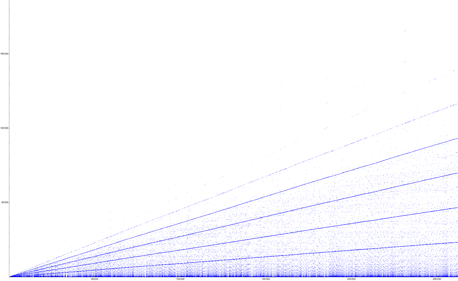
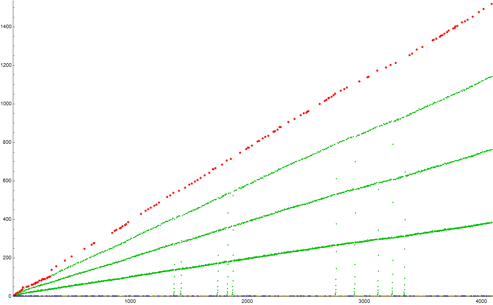
Figure 1.1 is a scatterplot of a(n) for 1 ≤ n ≤ 210. (Click here for an extended scatterplot of a(n) for 1 ≤ n ≤ 218).
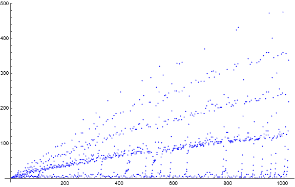
We note the following remarkable features of the scatterplot:
1. Quasi-radial striations (S) that appear to be evenly spaced.
a. Apparent even spacing.
b. Reflections of the original striation we call “S0”, which is that striation composed of the smallest terms.
c. Striation S1 appears to be the most dense, with subsequent echos S(ℓ) attenuating as ℓ increases.
d. Records often seem to attempt to build a new striation as n increases.
2. Catastrophes where the terms struggle to regain the quasi-radial pattern.
3. A “wood grain” appearance among the catastrophic progressions (evident in the extended scatterplot).
4. A subtle horizontal streaking in aggregate data associated with the frequency of values of τ(m) that result from Condition 0.
(Codes 2 and 3 generate analytical auxiliary sequences that enable study in this paper.)
Let Condition 0 pertain to novel a(n) and let Condition 1 pertain to extant a(n) = a(k) for 1 ≤ k < n. Thus we might define sequence b as a record of the conditions deployed by the algorithm behind a:
0, 1, 0, 1, 0, 1, 0, 1, 0, 1, 1, 0, 1, 0, 1, 1, 1, 0, 1, 1, 0, 1, 1, 0, 1, 1, 0, 1, 1, 1, 0, 1, 0, 1, 1, 1, 0, 1, 0, 1, 1, 1, 0, 1, 1, 1, 0, 1, 0, 1, 1, 1, 1, 0, 1, 1, 1, 0, 1, 0, 1, 1, 1, 1, 0, 1, 1, 0, 1, 1, 1, 0, 1, 1, 1, 0, 1, 1, 1, 0, 1, 1, 0, 1, 1, 1, 1, 0, 1, 1, 0, 1, 1, 1, 0, 1, 1, 1, 0, 1, 0, 1, 1, 1, 0, 1, 1, 1, 1, 0, 1, 1, 1, 0, 1, 0, 1, 1, 1, 1, ...
Therefore, a(1) and a(3) are novel and a(2) is extant i.e., a(2) appears at a(k) for 1 ≤ k < n, namely a(1) = a(2), etc. hence b(1) = b(3) = 0 and b(2) = 1. We can take indices j of 0s or 1s in b to identify the instigating condition that generates a(n+1).
Generally, Condition 0 has the effect of a(n) → a(n+1) nonincreasing, but normally represents a sharp decrease. Condition 1 has the effect of increasing a(n) → a(n+1) since the condition directive is the sum of nonzero positive integers. Hence, outside of the first 2 occasions of Condition 0, whenever we see a fall in a, we have Condition 0. A rise between consecutive terms is a hallmark of Condition 1. Therefore we may break the sequence a into cycles that start with Condition 0 and then are followed by 0 or more Condition 1 mappings. These cycles have the following lengths:
2, 2, 2, 2, 3, 2, 4, 3, 3, 3, 4, 2, 4, 2, 4, 4, 2, 5, 4, 2, 5, 3, 4, 4, 4, 3, 5, 3, 4, 4, 2, 4, 5, 4, 2, 5, 3, 3, 5, 3, 5, 4, 3, 4, 3, 4, 3, 5, 3, 5, 4, 3, 5, 5, 3, 5, 4, 4, 4, 3, 4, 3, 5, 4, 4, 5, 4, 2, 8, 3, 5, 6, 3, 4, 4, 4, 4, 5, 4, 4, 4, 5, 6, 5, 4, 5, 2, 6, 5, 4, 3, 5, 6, 4, 4, 3, 5, 5, 4, 5, 4, 3, 4, 6, 4, 5, 3, 4, 1, 3, 5, 5, 6, 4, 5, 5, 4, 4, 3, 4, ...
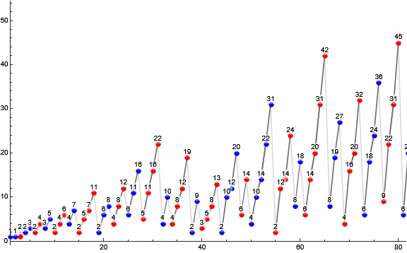
Figure 1.2 is a plot of a(n) for 1 ≤ n ≤ 80 showing even-indexed cycles in red and odd in blue. Condition 1 moves appear in dark gray lines and Condition 0 moves in light gray.
The maximum result of Condition 0.
Let r be the records transform of a. The sequence r begins:
1, 2, 3, 4, 5, 6, 7, 11, 12, 16, 22, 31, 42, 45, 52, 55, 64, 70, 74, 91, 92, 94, 100, 101, 110, 128, 130, 168, 188, 222, 248, 280, 289, 320, 329, 333, 370, 424, 432, 473, 476, 506, 524, 568, 588, 589, 630, 632, 641, 652, 680, 715, 726, 744, 776, 832, 836, 844, 872, 8802, ...
These appear at the indices n:
1, 3, 5, 7, 9, 12, 14, 18, 24, 27, 31, 54, 65, 80, 88, 110, 121, 132, 140, 166, 174, 186, 191, 199, 226, 239, 261, 267, 314, 359, 406, 485, 516, 548, 612, 632, 714, 832, 838, 952, 1003, 1080, 1117, 1193, 1246, 1267, 1359, 1369, 1398, 1426, 1449, 1503, 1585, 1591, 1662, 1776, 1853, 1880, 1949, 1985, ...
By definition of record, all terms in r, a(n) ≠ a(k) for 1 ≤ k < n. Hence, a(n + 1) = f(a(n)) = τ(a(n)). Therefore we may determine the maximum possible result T of Condition 0 by taking the length j of OEIS A2182 (recordsetters for τ(n)) such that M < a(n), where M is a term in A2182 and a(n) is in r. Then we find A2183(j), the maximum number of divisors given the most recent record in a.
The result of Condition 0 is a relatively small number 2 ≤ τ(m) ≤ T(n).
Table 2.1 is a description of the step-function T(n) for 1 < n < 219.
n T(n)
-------------
1 1
3 2
7 3
12 4
24 6
54 8
65 9
88 10
121 12
239 16
314 18
406 20
714 24
1585 30
1880 32
2679 36
3876 40
5467 48
11629 60
15895 64
21545 72
32813 80
36553 84
50770 96
86490 100
93230 108
93264 120
152066 128
158444 144
231357 160
303911 168
303985 180
304050 192
...
Records in a (outside of r = 1) arise from consecutive repetitions of Condition 1 that drive until terminated by a novel sum m that exceeds the previous record. Thereafter, Condition 0 pares down the function to τ(m) < m for novel m > 2. Therefore, for n > 3, records cannot occur consecutively, and a suffers a fall from its greatest height.
The prevailing low of the hopper sequence s.
Furthermore, we consider the smallest number u (i.e., the first term) in s even when it is not applied via Condition 1.
Let L(n) = max(L(k), L(n)) for 1 < k < n. Therefore L is nondecreasing while u may decrease.
Note that s generally maintains a prevailing low L except when Condition 0 yields a term m < L. This prevailing low L generally has multiplicity in s, and the distinct term L' in s that follows all the copies of L is comparable in magnitude to L such that when L is exhausted, oftentimes 1 ≤ L' − L ≤ 2. Hence, repeated iterations of Condition 1 yield m + L where L is nondecreasing but only increases by a small number 1 or 2. This is the source of the prominent quasi-radial striations seen in Figure 1.1.
Once m < L, m enters s before L and must be exhausted before making headway on the prevailing low L again.
Two modes of sequence a behavior.
We may distinguish two major modes of behavior of a using a characteristic function χ(n) = [L(n) − u(n) > 0], where the brackets are Iverson. Hence, if u has fallen below the prevailing low L, then χ(n) = 1, else χ(n) = 0. Furthermore, we may ignore the occasion of novel m → a(n) = τ(m). The resultant nonzero values of χ(n) constitute a “catastrophe” (C behavior) or falling away of the function a from primarily S (quasi-radial striation or echo) behavior.
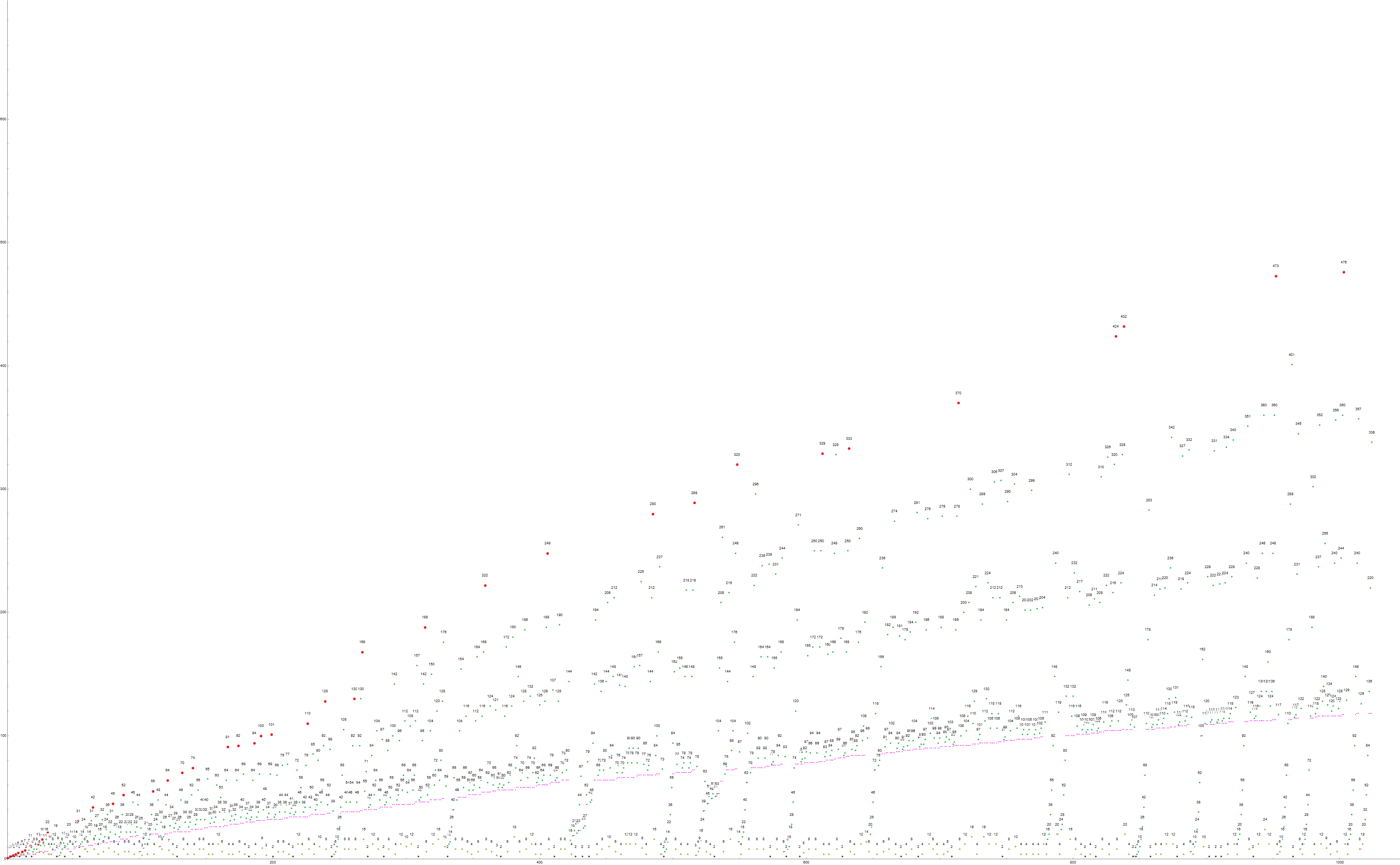
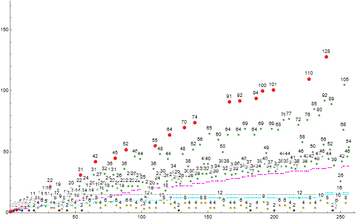
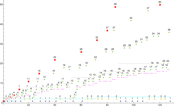
Figure 4.2 is a labeled scatterplot of a(n) for 1 ≤ n ≤ 29 highlighting in medium red markers n for which χ(n) = 1 resulting from Condition 1. Terms a(n) = τ(m) that result from Condition 0 are colored gold. We highlight in large green markers and label the index of the occasion of singleton instances of Condition 1. Records r are shown large, with prime records highlighted in cyan. (See Code 6; See an enlarged labeled scatterplot of a(n) for 1 ≤ n ≤ 212.)
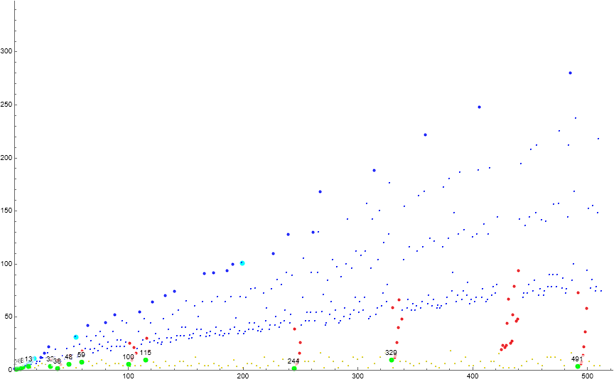
The distribution of gaps in coverage in a.
The sequence a is sensitive to the presence of m = a(k) for k < n, since the conditions concern novelty. Therefore we are interested in the occasion of gaps in coverage in a, i.e., values of m for which we may trigger the novelty Condition 0 and report the result of the payload function f(x).
Let z(n) be the mapping of [m ∈ a(1..n)] (brackets Iverson), hence z(n, m) = 1 if m appears in a(1..n) else 0 if it is absent or exceeds the current record. We may create an image of z.
Figure 5.1 is a plot of z(n, m) for 1 ≤ n ≤ 864, where black represents presence of m in a(1..k) for 1 ≤ k ≤ n, and white absence:
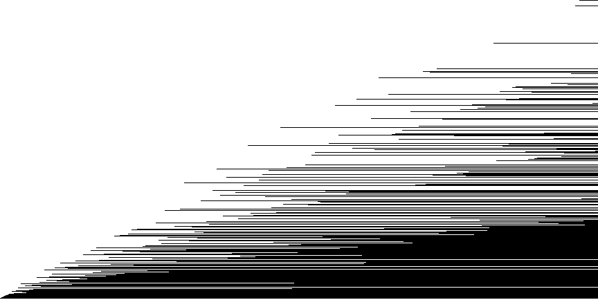
The function z which represents the presence of m in a establishes three major regimes as m increases. Having established the minimum of a at m = 1, for 1 ≤ m < c where c represents the least m not in a, we are assured Condition 1. For r < m, where r is the most recent record, we are assured Condition 0. For c ≤ m ≤ r, either condition may result, however, Condition 1 is liable to occur for m at the lower end of the range, while Condition 0 is more common as m approaches the record.
Let c(n) be the greatest integer such that all smaller nonzero integers can be found at a(k) for some 1 ≤ k < n. In other words, c(n) is the least (positive) m missing from a. Hence 1 ≤ m < c(n) assuredly instigates Condition 1, i.e., m already appears in a. This step function seems to stick for certain values; for sufficiently large n, this appears to be an artifact of the nature of the divisor counting function, specifically borne out in OEIS A5179. Some values of τ(n), namely large prime values, appear rarely.
Table 5.1 lists the first index n ≤ 219 where c takes a distinct value. (See Code 8.)
n c(n)
------------
1 2
3 3
5 4
7 5
9 6
12 7
14 8
21 9
39 13
43 14
49 15
423 17
4792 43
74111 171
313908 173
...
Figure 5.2 is a scatterplot of the number of gaps present in z(n) for 1 ≤ n ≤ 216. The function jumps at each record r and generally declines between them.
We may produce a similar function μ(n, m) that increments when m is encountered at a(k) and hence registers the number of times m has appeared in a(1..n).
The commonest number m in a(1..n) is m = 1 at n = 1, m = 2 for n = 6, m = 4 for n = 96, and m = 8 for n = 175552. Appendix Table A1 is more detailed and describes transition zones. Table A2 shows the 3 most common m for n = 2k and 3 ≤ k ≤ 19.
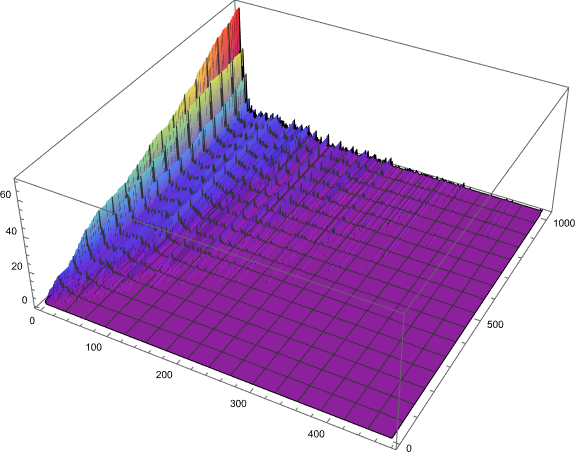
Figure 5.3 is a three-dimensional scatterplot of a(n) for 1 ≤ n ≤ 210 showing the multiplicity of m in a(1..n) as n increases. The color function and vertical height represents multiplicity. The m axis proceeds from the lower left corner toward the bottom. The n axis appears at right. The 5 most common terms are {4, 8, 2, 6, 12} in that order for n = 1024.
Singleton instances of Condition 0.
We note that c(n) > T(n) for n in the ranges (1..238), (4792..5466), (74111…?). Therefore, any Condition 0 result in these ranges will instigate Condition 1 thereafter, while outside these ranges, we might have repeated instances of Condition 0. Hence we might consider n in {239, 4792, 5467, 74111, …} in the light of these phase changes.
Figure 6.1 is a plot of the step functions c(n) (black, cf. Table 5.1) and T(n) (cyan, cf. Table 2.1) for 1 ≤ n ≤ 219. It is intermittently forbidden to have a repeated Condition 0 because the smallest gap in coverage c(n) > T(n), the largest possible number of divisors of the record r furnished by Condition 0.
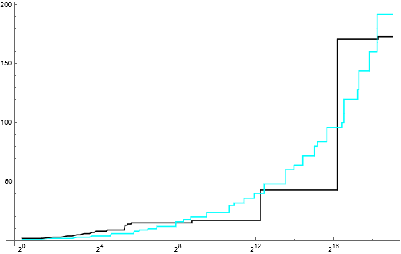
We note that for 1 ≤ n ≤ 219, Condition 0 repeats just once:
a(422) = 144, new to a. a(423) = τ(144) = 15, also new to a.
There is intermittent latitude to have a repeated Condition 0. What would be necessary is the emergence of a novel highly divisible instigator m such that τ(m) > c(n). Therefore, for 239 < n < 4791, it might be possible to obtain a novel highly divisible m that produces a novel τ(m) to furnish τ(τ(m)) thereafter. We might conject that the suppression of the possibility for n < 240 might have precluded the easy emergence of repeated Condition 0, though it may be that we could find another instance of repeated Condition 0 for n > 218 as the window to such has opened again at n = 74111.
Furthermore, we observe that large highly divisible numbers m often have even τ(m), since the divisor counting function is the product of incremented multiplicities of distinct prime divisors, and the only way of having an odd product is if all the multiplicities are even. The parity of a is predominantly even. Repeated Condition 0 is therefore rare and more instances of such may emerge as n increases.
Table 6.1 lists the number of even and odd terms in a(n) for the interval 2(k−1) ≤ n ≤ (2k − 1), followed by the ratio of evens over odds. For k > 2, evens dominate the sequence. (See Code 10.)
k evens odds evens/odds
--------------------------------
1 0 1 0
2 1 1 1
3 3 1 3
4 5 3 1.66667
5 10 6 1.66667
6 26 6 4.33333
7 49 15 3.26667
8 105 23 4.56522
9 227 29 7.82759
10 388 124 3.12903
11 829 195 4.25128
12 1535 513 2.9922
13 3234 862 3.75174
14 6573 1619 4.05991
15 13218 3166 4.17498
16 27044 5724 4.72467
17 54148 11388 4.75483
18 109408 21664 5.05022
19 221322 40822 5.42164
...
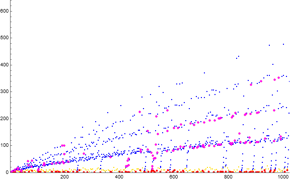
Figure 6.2 is a scatterplot of a(n) for 1 ≤ n ≤ 210 highlighting terms arising from odd Condition 0 progenitors in red, odd Condition 1 progenitors in magenta. Even Condition 0 progenitors are in gold and even Condition 1 progenitors are in blue.
Runs of Condition 1.
In contrast, runs of Condition 1 are the norm. For 1 ≤ n ≤ 218, there are 3273 occasions of singleton applications of Condition 1. For 1 ≤ n ≤ 219, there are 3273 occasions of singleton applications of Condition 1.
Table 7.1 shows the index n of run length ℓ of Condition 1, which is the i-th run of that parity. (See Code 9.)
ℓ i n
-------------------
1 1 2
2 5 10
3 7 15
4 18 50
5 72 262
6 133 531
7 69 246
8 125 493
9 144 585
10 203 847
11 465 2105
12 670 3073
13 1079 5085
14 1758 8492
15 1832 8871
16 3126 15370
17 1022 4793
18 5656 28602
19 10198 52200
20 14834 77276
21 24794 131549
22 35223 188984
23 53096 289168
24 70876 389535
...
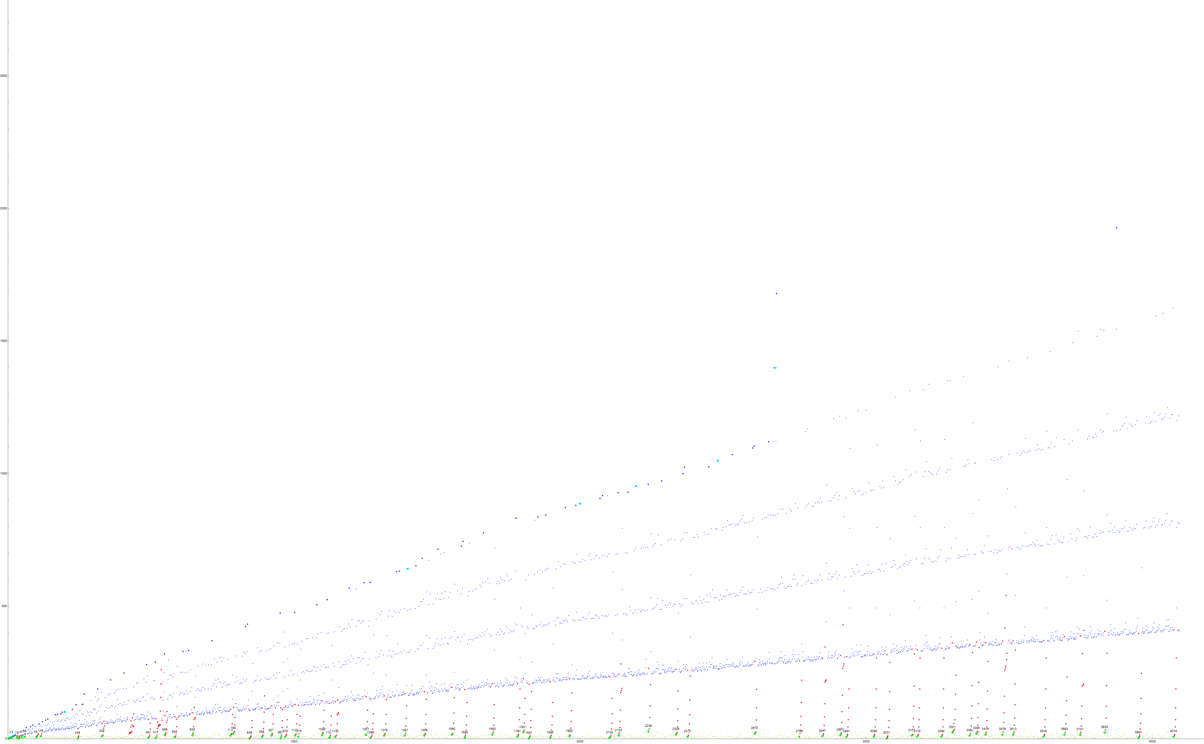
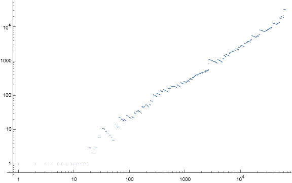
Figure 7.2 is a labeled scatterplot of a(n) for 1 ≤ n ≤ 28. Records a( j) = r appear in red, m = 2 following novel primes in blue, terms τ(m) instigated by novel m in gold and terms u + m by extant m in green. We mark the least term u in s in magenta, the greatest possible value T of τ(m) in cyan, and c(n) in black. See an extended labeled scatterplot of a(n) for 1 ≤ n ≤ 210, an unlabeled scatterplot of a(n) for 1 ≤ n ≤ 218, and a log-log scatterplot of a(n) for 1 ≤ n ≤ 210.
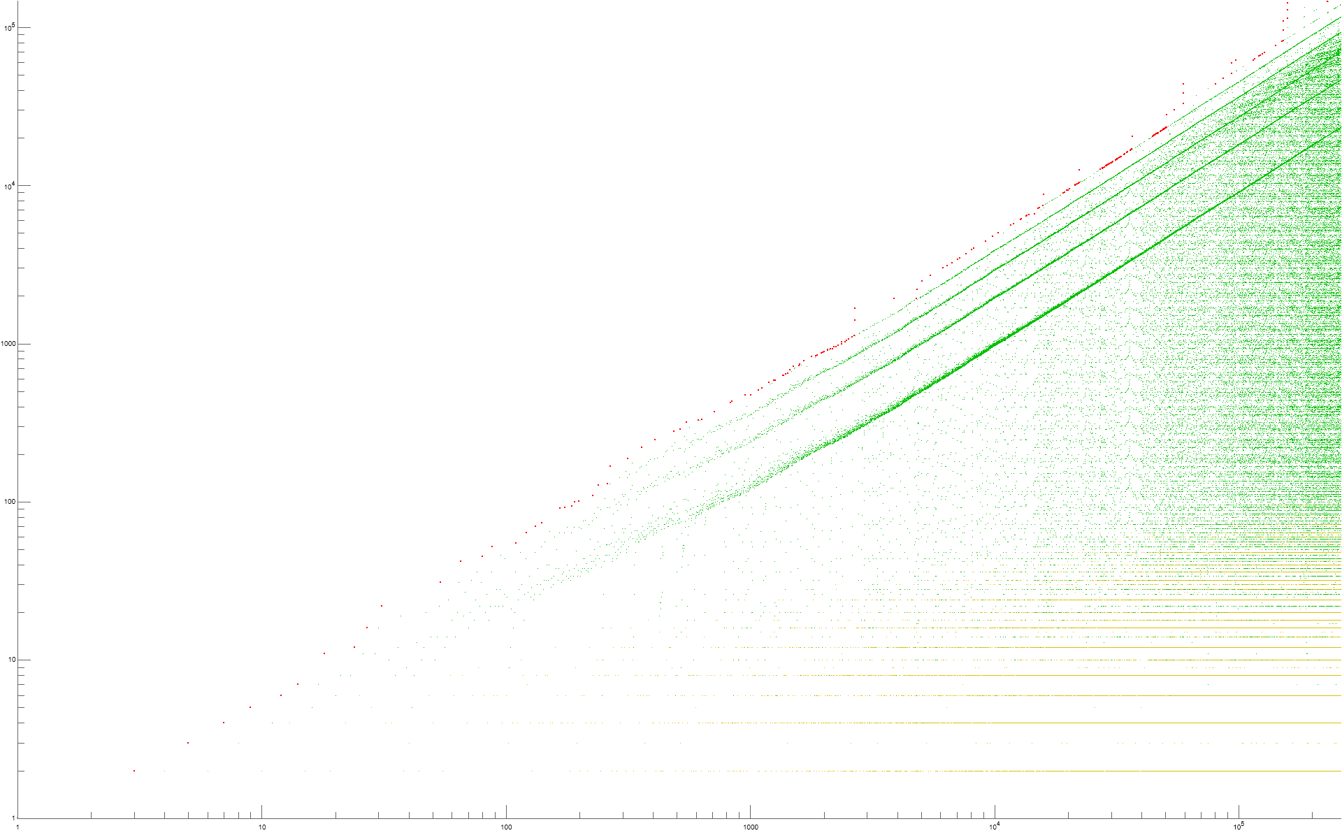
The results τ(m) of Condition 0 appear at the bottom of Figure 1.2 in gold, which comprise S0. By definition of T (the maximum value of the divisor counting function given the most recent record), these occupy the zone on or below the cyan line that represents T(n).
The magenta line represents u(n). The quasi-linear appearance is illusory; u(n) dips to respond to terms m < L, but it is L that appears linear. Terms in S1 appear above the magenta line, a reflection of S0 via Condition 1 (m + u). Subsequent repetitions of Condition 1 produce S2 and generally S(ℓ) for ℓ > 0.
Catastrophes.
We apply the term “catastrophe” to an episode in a where a(n) is brought very low, especially in the wake of a novel prime p, causing u to plummet below L and claw back after several consecutive iterations of Condition 1. We may delimit the catastrophe to occasions arising from Condition 1 for which L(n) − u(n) > 0, that is, when χ(n) = 1.
Catastrophic behavior (C) is apparent as a break in the general striation (S) pattern of the scatterplot, with a string of small terms rising back to S1 from S0. A conspicuous example begins at a(243) = 89, the first occasion of Condition 1 with run length ℓ = 7. Figure 1.2 shows that the lion’s share of catastrophes involve a singleton instance of Condition 1, or, rather, Condition 0 followed by Condition 1 followed by Condition 0 then a run of instances of Condition 1.
We note that manifestations of repetitions of Condition 1 feature u < L until such u is exhausted, therefore do not contribute to the quasiradial striations. This is the source of “out of place” points that do not lie in the striations. In these occasions we see (m + u) = (a(n) + a(n − 1)), that is, the sum of adjacent most recent small terms. Hence we may see a subsequence such as one triggered novel prime p → 2 → novel squarefree semiprime → 4 → 6 → 10 → 16 → 26 → 42 → etc. so long as all those terms exist in a. (This particular subsequence is triggered by a(243) = 89.)
We associate catastrophes to singleton instances of Condition 1 in all instances except the single observed occasion of a repeated instance of Condition 0 at a(422..423). Catastrophes sometimes occur in the wake of records. Prime records do not seem to necessarily trigger catastrophes.
Let’s trace the precipitation of a catastrophe. We write Condition 0 as “→” and Condition 1 as “⇒”. Terms resulting from Condition 1 appear in blue, from Condition 0 in a warm color, but novel primes appear in orange, records in red.
The usual mode of catastrophe is via singleton Condition 1.
Suppose we have m ⇒ (u + m) extant. Then we have Condition 1 following Condition 1, and thus (u + m) ⇒ (u + m) + m if m ≤ L, or (u + m) ⇒ (u + m) + L if m ≥ L. If the former, we have a Fibonacci-like cycle wherein Condition 1 reports (a(n) + a(n−1)), that is, the sum of the two latest preceding terms, since a(n−1) < L and thus must be consumed first from the hopper. This cycle continues until the sum meets or exceeds L. This is the catastrophic (C) pattern, sustained until u ≥ L.
Thereafter we have the latter echo pattern, i.e., m ⇒ (u + m) ⇒ (u + m) + L with m ≥ L. The echos are only false since L is not necessarily consistent; we exhaust u = L, therefore we might run out of copies of the prevailing low L and begin to consume a slightly larger L.
If Condition 1 immediately enters (m + u) ≥ L, we have the striation or echo pattern (S), since a point in striation S0 is echoed in striation S1 via (u + L). This subtends j times, making j echos with the final point at Sj, and terminates when we have a novel sum and thus Condition 0.
If Condition 1 enters (m + u) < L then the function a languishes in the Fibonacci-like cycle until the sum (m + u) ≥ L, and thereafter the echo involves a point not in S0, therefore the points resulting from the catastrophe are likely “off grid” regarding the striations. By these we have up to two phases of catastrophe. The first phase involves the introduction of u < L and the Fibonacci-like cycle. Sometimes a sum may prove novel and thus terminate the cycle in this first phase. Otherwise, at some point the sum meets or exceeds L, introducing u ≥ L, and thereafter we have cured and are again making headway against the stock of copies of L and then larger L. Hence, a Fibonacci (C1) and a cured, echo phase (C2).
An example of (S): a(17) = 7:
7 ⇒ 11 → 2 ⇒ 6 ⇒ 8 → 4 ⇒ 8 ⇒ 12 → 6 ⇒ 11 ⇒ 16 → 5 ⇒ …
We begin with the extant 7 and add the prevailing low 4 (multiplicity is 3) to obtain 11, consuming a 4. The record prime 11 furnishes 2, triggering a catastrophe since 2 < 4, therefore after a(20) = 2 + 4 = 6, we have a Fibonacci cycle that immediately yields novel 8 and interrupts the C1 phase. In this case, the subduction of 2 below prevailing low 4 is immediately cured in the next term because the C1 cycle yields m > L (but in this case was also killed by a new m). We have consumed 1 copy of the two 4s, but restore a 4 at a(22), exhausting L = 4 at a(24) = 12 (a record). The high Condition 0 result 12 ⇒ 6 means that we continue to make headway against L = 5 thereafter, to reinforce L = 5 with the occasion of a(27) = 6. Throughout this example, s either cured or always exposed the prevailing low L to deployment via Condition 1.
Singleton Condition 1 results in typical catastrophic behavior. The example is the 12th Condition 1 catastrophe which starts at a(243). Here, the hopper s contains the following numbers, their multiplicities superscripted:
{372, 388,405, 41, 423, 446, 45, 463, 482, 49, 502, 523, 55, 562, 58, 60, 644, 65, 68, 693, 70, 72, 74, 762, 77, 80, 85, 89, 91, 922, 94, 100, 101, 110, 128}
Hence L = 37 with a multiplicity of 2. We start at a(242):
52 ⇒ 89 → 2 ⇒ 39 → 4 ⇒ 6 ⇒ 10 ⇒ 16 ⇒ 26 ⇒ 42 ⇒ 68 ⇒ 105 → 8 ⇒ 46 ⇒ …
a(242) = 52 reinforces the 2 copies of 52 in s, consuming one of 4 copies of 37 in s to furnish novel prime 89. The novel prime triggers Condition 0 and reports 2 < 37. The number 2 has appeared many times, triggering Condition 1 and reporting 2 + 37 = 39. We place 2 at the head of s to be consumed first in the next occasion of Condition 1. The new 39 triggers Condition 0 and reports 4; 39 slips into s after {2, 37, 38, 38}. The number 4 has appeared many times therefore we have Condition 1 and consume 2 + 4 = 6, entering the Fibonacci cycle (phase C1) through a(252) = 68, which is extant and still triggers Condition 1. Since the previous term 42 > 37, we enter phase C2, and report a novel a(253) = 105.
Therefore, we see that the behavior of the C1 phase involves the singleton Condition 1 trigger and the first Condition 1 trigger after the interposing Condition 0. These become the first terms of the Fibonacci behavior. In this example, these terms are (2, 4) and we can consequently use these terms as a signature for the catastrophe. The signature (2, 4) appears in the list of Condition 1 catastrophes at the following indices:
12, 41, 199, 527, 533, 770, 945, 1022, 1124, 1148, 1167, 1201, 1219, 1381, 1535, 1589, 1606, 1755, 1757, 1828, 1937, 2014, 2207, 2326, 2455, 2556, 2673, 2760, 2831, 2895, 3168, 3184, 3353, 3381, 3506, 3574, 3584, 3631, 3754, 3772, 3953, 4002, 4062, 4203, 4234, 4427, 4445, 4465, 4477, 4861, 4916, 5208, 5249, 5374, 5378, 5379, 5477, 5546, 5601, 5603, 5613, 5633, 5781, 5880, 5883, 5945, 6028, 6095, 6411, 6497, 6534, 6607, 6631, ...
The corresponding indices of the singleton Condition 1 triggers for signature (2, 4) catastrophes are the following (see Code 7):
244, 1821, 15595, 45312, 45920, 63497, 78944, 85896, 93712, 95206, 96661, 100207, 101609, 113048, 125269, 129108, 130355, 140198, 140299, 146922, 156671, 161845, 178893, 189446, 198863, 206914, 215596, 222057, 226882, 231865, 254325, 255139, 268845, 270532, 279983, 285547, 286181, 289942, 298280, 299598, 315705, 319537, 323355, 334011, 336447, 354012, 355274, 356892, 357799, 387205, 390687, 413863, 416197, 427380, 427610, 427694, 436251, 441956, 445363, 445426, 446409, 447960, 458041, 465117, 465353, 470119, 476674, 481367, 506947, 513824, 516469, 520731, 522585, ...
The commonest signature is (8, 4) for n ≤ 219. See Code 5.
The next instance of (2, 4) catastrophe is the 41st Condition 1 catastrophe starting at a(1821):
414 ⇒ 617 → 2 ⇒ 205 ⇒ 4 ⇒ 6 ⇒ 10 ⇒ 16 ⇒ 26 ⇒
42 ⇒ 68 → 110 ⇒ 178 ⇒ 288 ⇒ 466 → 4 ⇒ 207 ⇒ …
When similar signatures appear near one another in the scatterplot they have the appearance of “chatter” or a sort of resonance, since the same numbers appear in the first part of the catastrophe. A later instance of the same signature makes more progress in the Fibonacci (C1) phase unless it is quite soon after, since L is nondecreasing. However, a later instance of the signature catastrophe is longer, since it will find a new novel termination, having already discovered all the terms in its subsequence in a.
The effect of Condition 0 is to report τ(m), i.e., novel m → τ(m), τ(m) ≤ m for n > 3. We observe the intermittent possibility of T(n) > c(n) so as to admit the entrance of repeated Condition 0, (first) instigated at a(421):
80 ⇒ 144 → 15 → 4 ⇒ 19 ⇒ 23 → 2 ⇒ 21 ⇒ 23 ⇒ 44 ⇒ 67 →
2 ⇒ 25 ⇒ 27 ⇒ 52⇒ 79 → 2 ⇒ 46 ⇒ 48 ⇒ 94 ⇒ 142 ⇒ 194 → 4 ⇒ 68
In this range the prevailing low L = 64 with multiplicity 9 in s. Condition 0 maintains L = 64 since u is not applied to the function. After the two iterations of Condition 0, a(424) = 4 → u, now 4 appears at the head of the hopper s ahead of the 9 copies of 64. Repeated iterations of Condition 1 thereafter must consume this u < L until (m + u) ≥ L. Consequently, repeated Condition 1 operates as a Fibonacci-like sum of the most recent two terms until the sum is equivalent to or exceeds L. Thereafter, Condition 1 makes headway on the stockpile of L until (m + u) is not in a and we have Condition 0 thereafter. In the case of the catastrophe in the wake of a(422..423), several cycles of Condition 1 interrupted by singleton Condition 0 follow until u(442) = L(442) = 64.
The trigger for this unique catastrophe is the subduction of u < L at a(423), and its intensification at a(424) = 4.
The occasion of catastrophes appears more or less evenly as n increases, but with notable dearths. These are not necessarily associated with the “phase changes” wherein the maximum result T(n) of Condition 0 is less than the largest contiguous extant term c(n).
Conspicuously, there is a catastrophe instigated by the doubled instance of Condition 0 starting with novel a(422) = 144 → τ(144) = 15 → τ(15) = 4 ⇒ 15+4 = 19 ⇒ 19+4 = novel 23 → τ(23) = 2 ⇒ 2+19 = 21, etc.
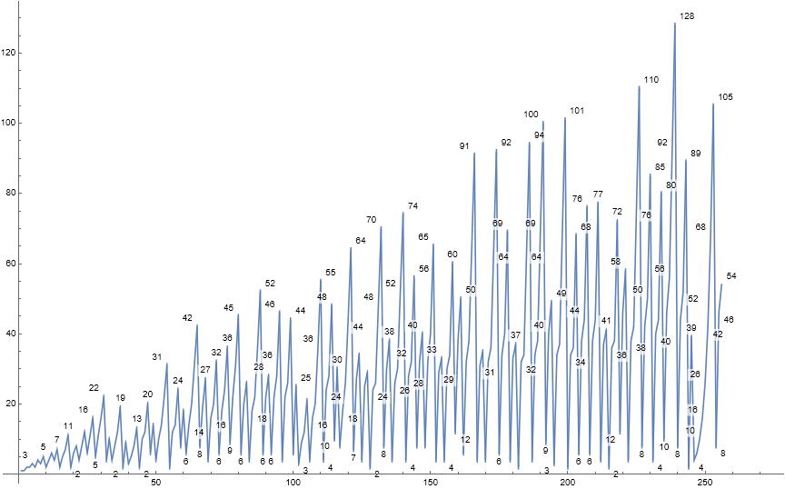
Figure 8.1 is a labeled plot of a(n) for 1 ≤ n ≤ 28. The catastrophe beginning with a(243) = 89 is conspicuous at right.
Fibonacci phase (C1) of catastrophic progressions.
Finally, we address the “wood grain” appearance among terms that result from runs of repeated applications of Condition 1 when u < L.
It is perhaps easy to see this pattern when we merely plot u(n). We have already described the fall of a(n) instigated by a novel m for which τ(m) < L, hence, u < L. It is likely before long, citing the step behavior of c(n), that all or nearly all common small values of τ(a(n)) ≤ T(n) appear in a and thus trigger Condition 1. If we have the Condition pattern 0, 1, 0, the second manifestation of Condition 0 yields a small m that enters a run of Condition 1 involving the sum of small adjacent terms. These runs are identical and appear throughout the sequence, only terminating with a novel m. Some of these conditions occur fairly often and therefore we have a “chatter” pattern among terms not arranged into the quasi-radial striations.
The scatterplot of u(n) aggregates all the C1 phases of the catastrophes in a.
Figure 9.1 is a labeled scatterplot of u(n) for 1 ≤ n ≤ 216 in purple, L(n) in magenta, T(n) in cyan, and c(n) in black.
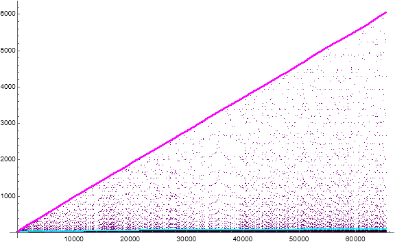
We observe that the singleton Condition 1 term a(n) = m is followed by a Condition 0 term (m + u) which yields the first term τ(m + u) of a run of Condition 1 terms in catastrophe. Since m → u if m < L(n), we have Condition 1 furnish the sum of adjacent most recent terms until we encounter a novel sum.
Hence, the Condition 1 catastrophe can be classified by the terms (m, τ(m + u)). The first Condition 1 catastrophes have the following signatures:
(1, 2), (2, 2), (2, 3), (3, 2), (4, 2), (4, 4), (2, 3), (6, 4), (8, 6), (6, 3), (10, 8), (2, 4), (10, 2), (4, 2), (3, 6), (14, 4), (6, 2), (14, 6), (12, 4), (20, 4), (2, 2), (6, 4), (12, 4), (4, 6), (8, 4), (12, 4), (8, 12), (15, 4), (4, 4), (8, 2), (15, 4), (4, 2), (12, 4), (12, 8), (12, 4), (16, 2), (4, 4), (16, 6), (8, 4), (24, 4), (2, 4), (4, 4), (10, 2), (4, 2), (12, 6), (28, 8), (16, 4), (8, 2), (20, 2), (8, 12), (10, 4), (14, 4), (8, 4), (8, 4), (2, 2), (12, 2), (8, 4), (8, 4), (24, 3), (12, 8), (20, 4), (16, 4), (16, 10), (16, 6), (8, 4), (16, 8), (15, 6), (24, 10), (4, 2), (8, 4), (24, 2), (12, 8), (16, 4), (20, 8), (8, 6), (8, 2), (15, 2), (2, 2), (9, 4), (2, 8), (16, 2), (24, 4), (2, 2), (8, 4), (8, 4), (12, 4), (24, 4), (8, 4), (8, 8), (10, 4), (40, 4), (8, 2), (8, 2), (4, 6), (18, 4), (8, 8), (12, 6), (12, 2), (12, 8), (8, 8), (36, 12), (8, 4), (12, 8), (16, 6), (12, 12), (16, 4), (12, 18), (24, 4), (16, 4), (12, 4), (12, 4), (18, 2), (18, 2), (32, 2), (24, 2), (8, 4), (21, 4), (12, 2), (36, 12), (12, 6), ...
We note that (1,2) is unique, since 1 appears in a twice, its second appearance the only Condition 1 appearance. The catastrophe starting with a(243) has signature (2,4). Hence its unimpeded progression would be {2, x, 4, 6, 10, 16, 26, 42, 68, 110, …} where x triggers Condition 0 and in this case, must be a squarefree semiprime to obtain τ(x) = 4.
Because we can identify a signature that instigates a Fibonacci-like subsequence until exhaustion at novel sum, we read subsequences with the same signature in a scatterplot as “chatter” or the wood-grain appearance.
Proof of an infinite sequence a.
The sequence is infinite. A number m is either new to a or it is not. Thus, we will have Condition 0 which yields τ(m) or we will have Condition 1 that yields the sum (m + u). The arithmetic of a is among positive integers m, and there is always an integral τ(m) ≥ 1. The number m = 1 appears exactly twice in a and never again, since 1 can only be extant after its first appearance, which triggers the sum 1 + u, where u ≥ 1. Therefore, for n > 3, u ≥ 2 ← τ(p) for novel prime p. We note that the hopper s that contains the sorted list of terms in a that have not been expended by extraction of the then-smallest term u has a length ℓs that increments upon exercise of Condition 0, therefore ℓs is nondecreasing. Effectively, ℓs is a record of the number of times Condition 0 has played for a(n). This nondecreasing ℓs implies that there will always be a least term u of s by which we might exercise Condition 1 (m + u) ≥ 4 for n > 3. The consecutive repetition of Condition 1 that involves the summation of the last two terms (a(n) + a(n−1)) proceeds until the sum is novel, gradually covering a relatively small range and forcing longer runs of Condition 1 as n increases, since the supply of gaps in s becomes more rarified above c(n). Records arise from consecutive repetitions of Condition 1 that drive until terminated by a novel sum that exceeds the previous record. Therefore we conclude that a is an infinite sequence.
On an analogous sequence a'.
Let us examine a similar sequence a' that substitutes the payload function f(x) = τ(x) with ω(x + 1). We note that a sequence that uses ω(x) has cardinality 2, i.e., {1, 0}, and if we should begin with the first term 2, it has cardinality 3, hence we introduce the increment so as to provide for an infinite sequence. Hence Condition 0 reports ω(m + 1) and Condition 1 reports (m + u) for m = a'(n).
The sequence a' begins:
1, 1, 2, 1, 2, 3, 1, 3, 4, 1, 3, 4, 7, 1, 4, 5, 2, 5, 7, 11, 2, 6, 1, 3, 4, 7, 11, 15, 1, 6, 7, 12, 1, 7, 8, 1, 7, 8, 15, 22, 1, 8, 9, 2, 9, 11, 18, 1, 8, 9, 17, 2, 10, 1, 3, 4, 7, 11, 18, 26, ...
The local low is 1 throughout the sequence since prime (n + 1) →1 through Condition 0. The reduction of m via Condition 0 = ω(m + 1) is more severe than the τ(m) formulation. Because of this, the function a' persists in the (S) pattern (i.e., Condition 1), with relatively few catastrophes induced by ω(m + 1) → u < L given a low value of m that results from a single iteration of Condition 1. The catastrophes (C1) still precipitate Fibonacci chains via the subduction of u < L and enter post-catastrophe (C2) phase usually out of sync with the general quasi-radial striations. We see the same echoing of S0 into higher striations.
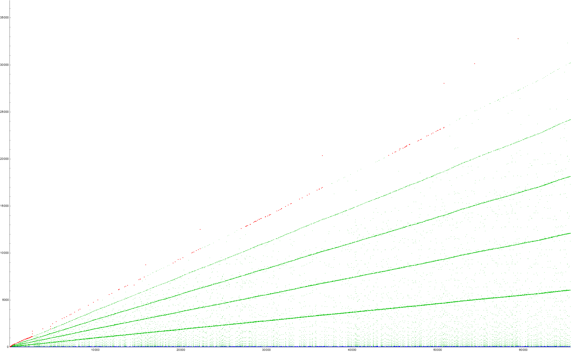
Figure 10.1 is a scatterplot of a'(n) for 1 ≤ n ≤ 212. Records are in red, terms instigated by Condition 1 in green, Condition 0 in gold, and local minima (i.e., m = 1) in blue.
The few catastrophes are evident in Figure 10.1, in an otherwise crisper field of quasi-radial striations.
Figure 10.2 is a labeled scatterplot of a'(n) for 1 ≤ n ≤ 27 akin to Figure 7.2. Records a( j) = r appear in red, m = 1 following novel m for which (m + 1) is a prime power in blue, terms ω(m) instigated by novel m in gold and terms u + m by extant m in green. We mark the least term u in s in magenta, the greatest possible value T of ω(m) in cyan, and c(n) in black.
Sticky gap m = 3257 after a'(36152).
We have found no occasions of repeated Condition 0 for 1 ≤ n ≤ 65536. Repeated Condition 0 is forbidden outside of the first 2 terms, since c(n) > T(n) to a harsher degree than in a, where there was a closer balance. This sequence (a' ) fills gaps quickly compared to a: the smallest gap in a' (1..1261) is 137, which appears at a' (1373), whereas m = 131 has not appeared in a for n ≤ 524288.
However, we see that m = 3257, the 460th prime and smallest gap for n > 36152, has not yet appeared given 131072 terms of a'. Are there “sticky” gaps, or is 3257 merely the first of many m not in a' ? If 3257 does not appear due to Condition 1 (i.e., via the sum (m + u)) then perhaps it might if a new m appears with 3257 distinct prime factors. Condition 1 certainly is the source of gap-filling m as well as records for n > 1. It would seem that at some point, 3257 will appear in a' through Condition 1 as well. If m = 3257 appears in a such that T(n) > 3257, it might trigger repeated Condition 0.
Additionally, the second gap freezes after a similar roughly linear escalation. Perhaps a' does not cover the range m.
The enumeration of gaps of coverage.
Suppose we have a number m missing from a sequence f(1..n), and suppose it is the first of a run of ℓ missing numbers such that they form a gap containing {m, m+1, m+2, …, m+ℓ−1}. We may annotate this gap in an ordered pair (m, ℓ). We may describe the presence and absence of any m in f by sorting a list G of (m, ℓ) according to m. We presume a minimum for f (through preliminary analysis) and therefore have a final ordered pair with greatest m thus: (m, ∞), since no m appears in f(1..n) that exceeds the most recent record. Hence we may enumerate the gaps in f(1..n) using a function g(n). Likewise, we may ascertain the least gap c(n) = the least m in G and the most recent record r = (m − 1) such that ℓ = ∞, i.e., 1 less than the greatest m in G. If the sequence f(1..n) covers m ≤ r, then there is one ordered pair in G, that is, (r + 1, ∞), hence c = r + 1. The number g then counts voids in coverage of m by f. (See Code 11, which is written according to this principal, though Code 8 is an expedited but limited method for ascertaining c.)
Let g pertain to a and g' to a'.
The sequence g begins:
1, 1, 1, 1, 1, 1, 1, 1, 1, 1, 1, 1, 1, 1, 1, 1, 1, 2, 2, 2, 2, 2, 2, 2, 2, 2, 3, 3, 3, 3, 4, 4, 4, 4, 4, 4, 5, 5, 4, 4, 4, 4, 4, 4, 4, 4, 4, 4, 4, 4, 4, 4, 4, 5, 5, 5, 5, 6, 6, 6, 6, 6, 6, 6, 7, 7, 7, 8, 8, 8, 8, 8, 8, 8, 8, 9, 9, 9, 9, 10, 10, 10, 10, 10, 10, 10, 10, 11, 11, 11, 11, 11, 11, 11, 11, 11, 11, 11, 11, 11, 10, 10, 10, 10, 9, 9, 9, 9, 9, 10, 10, 10, 10, 11, 11, 11, 11, 11, 11, 11, ...
The sequence g' begins:
1, 1, 1, 1, 1, 1, 1, 1, 1, 1, 1, 1, 2, 2, 2, 2, 2, 2, 2, 3, 3, 2, 2, 2, 2, 2, 2, 3, 3, 3, 3, 3, 3, 3, 3, 3, 3, 3, 3, 4, 4, 4, 4, 4, 4, 4, 5, 5, 5, 5, 5, 5, 4, 4, 4, 4, 4, 4, 4, 5, 5, 5, 5, 5, 5, 5, 5, 5, 5, 5, 5, 6, 6, 6, 5, 5, 5, 5, 5, 6, 6, 6, 6, 6, 6, 7, 7, 7, 6, 6, 6, 6, 7, 7, 7, 7, 7, 8, 8, 8, 8, 9, 9, 9, 9, 8, 8, 8, 8, 8, 9, 9, 9, 9, 10, 10, 10, 10, 10, 10, ...
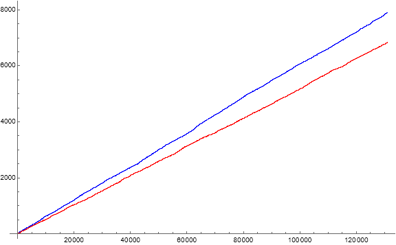
Figure 10.3 is a scatterplot of the number of gaps g(n) in a(1..n) in blue and g'(n) in a'(1..n) in red for 1 ≤ n ≤ 217.
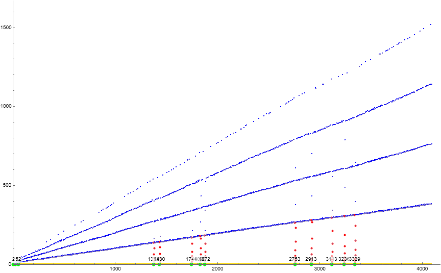
2, 21, 52, 1372, 1430, 1744, 1828, 1872, 2753, 2913, 3113, 3236, 3339, 4136, 4225, 4309, 5366, 5914, 6619, 6754, 6914, 6942, 6990, 7338, 7403, 7729, 8007, 9207, 9521, 9961, 10250, 10281, 10550, 12321, 12493, 12947, 13074, 13314, 13583, 13737, 13990, 14407, 14484, 14559, 14582, 14647, 14933, 15560, 15638, 16291, 16650, 17066, 17398, 17658, 18067, 18841, 19512, 20352, ...
These are the first terms of the occasions of u < L in sequence a', hence the triggers for catastrophe. The same sort of catastrophe signatures may be derived in analogy to those for a, such that catastrophes might be catalogued for a'.
Figure 10.4 is a labeled scatterplot of a'(n) for 1 ≤ n ≤ 212 highlighting in medium red markers n for which χ(n) = 1 resulting from Condition 1. Terms a'(n) = ω(m) that result from Condition 0 are colored gold. We highlight in large green markers and label the index of the occasion of singleton instances of Condition 1. This plot is analogous to Figure 4.2 which pertains to a.
The function a' appears to be more faithful to (S) behavior than a, with fewer catastrophes and a Condition 0 with a tighter range. The occasion of repeated Condition 0 seems completely prohibited in a'. The reluctance or complete absence of certain m in a' may or may not say something about similar issues in a, since the payload function f(x) = ω(m + 1) is impure in a'.
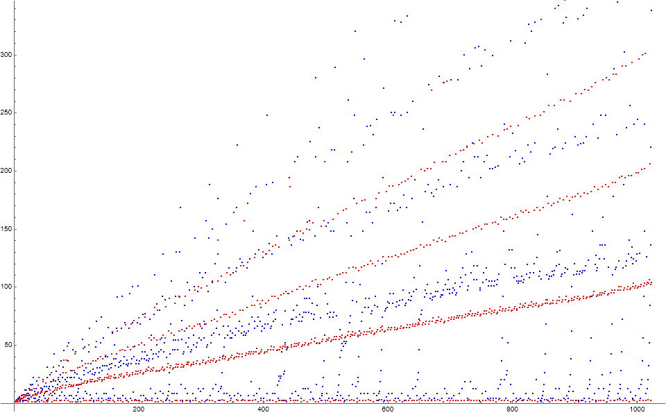
Figure 10.5 is a comparison scatterplot of a(n) (i.e., “tau”) in blue and a'(n) (i.e., “omega”) in red for 1 ≤ n ≤ 210.
Conclusions.
We have examined the principal features of OEIS A345147. Here is a summary.
- We may break the sequence a into cycles that start with Condition 0 and then are followed by 0 or more Condition 1 mappings. Generally, Condition 0 has the effect of a(n) → a(n+1) nonincreasing, but normally represents a sharp decrease. Condition 1 has the effect of increasing a(n) → a(n+1) since the condition directive is the sum of nonzero positive integers. Hence, outside of the first 2 occasions of Condition 0, whenever we see a fall in a, we have Condition 0. A rise between consecutive terms is a hallmark of Condition 1.
- Consider the “hopper” sequence s, a sorted version of a, from which we strike its least term u when it is applied through Condition 1. We develop a nondecreasing prevailing low L that normally has multiplicity in s. L is tantamount to the local maxima of s. The sequence a exhibits an echo behavior when m ≥ L, but suffers catastrophe when m → u < L. The prevailing low L is the consequence of the necessity to consume u, the least term in s, when applied by Condition 1.
- There are 3 regions of the range m. For 1 ≤ m < c, where c is the least m missing from a, we are assured Condition 1, thus, the sum (m + u) and “echoing” behavior. For m > r where r is the (most recent) local maximum, we are assured Condition 0 thus τ(m). For c ≤ m ≤ r, we may have either condition, though Condition 1 is more likely for m closer to c, and Condition 0 more likely for m closer to r. Of course, for m = c, we have Condition 0, and for m = r we have Condition 1.
- The minimum of a is 1 and for n > 3, 2 is the least available m. The term m = 1 appears twice in a; its second occasion a(2) is the result of τ(1), but 1 has already appeared, therefore we sum (1 + 1) = a(3) = 2. Thereafter we can never again see 1 because the least Condition 0 results from primes and the least sum from Condition 1 involves at minimum (m + 2). As a consequence, 3 also appears only twice in a.
- Condition 0 brings m → τ(m) relatively low while the Condition 1 summation (m + u) provides a ladder eventually to reach a relatively high term, m new to a. The extreme case for Condition 0 is of course the emergence of a prime p new to a, thus, p → τ(p) = 2. A novel prime does not necessarily precipitate a catastrophe, since terms that follow 2 are already in a.
- Echo behavior mode S. When Condition 1 iterates the first time in a cycle, its effect in bringing (m + u) ⇒ m high is minimal. This lands m in a part of the range such that Condition 1 is most likely. If Condition 1 does not yield a novel m, we produce a series of echoes a(n+1) = (a(n) + L), a(n+2) = (a(n+1) + L), …, a(n+k) = (a(n+k−1) + L) of a low term a(n) = m and have the quasi radial striations (S). Novelty is increasingly likely as m increases toward the record, above which it is certain to be new to a, ending the cycle. The striations S are not actually linear, since the prevailing low L, though it is nondecreasing, possesses finite multiplicity. Hence it is not assured that L remains the same during an (S) cycle, though L at the start and L once it changes have a small difference that is usually 1 or 2.
- Catastrophic behavior mode C. If Condition 1 iterates just once and discovers a low novel M, Condition 0 will pare it down such that M → (u < L). In all cases but 1 (i.e., a(422)) Condition 1 then resumes and enters into a cycle (C1) in which the sum (m + u) ⇒ (a(n) + a(n − 1)), i.e., the sum of the two most recent terms, or a Fibonacci cycle. The cycle terminates when m ≥ L and we enter (C2), the post-catastrophic cycle that normally echoes a term m that is not within the striations. Phase C1 may be interrupted by the discovery of a novel term, but eventually, C2 yields a term m new to a and the episode ends.
- The single (observed) occasion of a repeated Condition 0 begins with a(421) = 80, extant in a, then through Condition 1 (m + u) = (80 + 64) = a(422) = 144, new to a, through Condition 0, τ(144) = a(423) = 15, new to a, through Condition 0, τ(15) = a(424) = 4. The least term u languishes below L through subsequent adjacent Condition 1 catastrophes until n = 442. It seems likely that this occasion is the sole appearance of repeated Condition 0 in a.
- The Condition 1 catastrophes can be catalogued according to their signature, that is, the instigator of Condition 1 and the term that follows the interposing Condition 0. Catastrophes of the same signature follow the same Fibonacci cycle and make headway as they re-emerge. For instance, the catastrophe that begins at a(244) = 2 is followed by a(246) = 4, hence has signature (2, 4). The terms a(246..252) are 4, 6, 10, 16, 26, 42, and 68. The next term is 105 since, by that point, m > L, therefore (68 + 37) = 105, and the Fibonacci cycle C1 has ended. The next occasion of a signature-(2, 4) catastrophe appears at a(1821) and the C1 cycle proceeds further since L is greater, thus more of the terms, 110, 178, etc., enter a.
We have examined a similar sequence that substitutes the novel payload function f(x) = τ(x) with f(x) = ω(x+1). This sequence shares many features with a, and might say something about the appearance of certain m as n increases, which might merit further study.
This concludes our examination.
Appendix:
Table A1: Commonest terms m in a(1..n) and their transitions.
Range n Commonest m
---------------------------------------
( 1...3) 1
( 4...5) 2 & 1 (2 each)
( 5..33) 2
(34..37) 4 & 2 (6 each)
(38..83) 2
(84..91) 4 & 2 (9 each)
(92..95) 6, 4, & 2 (9 each)
(96...175324) 4
(175325...175341) 4 & 8 (6848 each)
(175342...175345) 4
(175325...175380) 4 & 8 (6849 each)
(175381...175409) 8
(175410...175418) 4 & 8 (6849 each)
(175319...175436) 4
(175437...175418) 4 & 8 (6850 each)
(175459...175479) 8
(175480...175484) 4 & 8 (6854 each)
(175485...175516) 8
(175517...175551) 4 & 8 (6855 each)
(175552...) 8
...
Table A2: List of the 3 most common terms m in a(1..n) for n = 2k and 3 ≤ k ≤ 19. Quantities precede the parenthetic term (m).
k 1st 2nd 3rd
----------------------------------------
3 3 (2) 2 (3) 2 (1)
4 5 (2) 3 (4) 2 (5)
5 6 (2) 5 (4) 3 (11)
6 9 (2) 7 (4) 5 (8)
7 13 (4) 10 (6) 10 (2)
8 25 (4) 15 (6) 14 (2)
9 36 (4) 27 (8) 24 (2)
10 70 (4) 46 (8) 44 (2)
11 130 (4) 83 (8) 69 (2)
12 235 (4) 174 (8) 131 (2)
13 440 (4) 333 (8) 224 (2)
14 824 (4) 683 (8) 416 (12)
15 1503 (4) 1322 (8) 832 (12)
16 2801 (4) 2606 (8) 1611 (12)
17 5303 (4) 5141 (8) 3063 (12)
18 10118 (8) 9974 (4) 5869 (12)
19 19749 (8) 18652 (4) 11956 (16)
Block[{a = {1}, s = {}},
Do[If[FreeQ[#2, #1],
AppendTo[a, DivisorSigma[0, a[[-1]] ] ],
AppendTo[a, a[[-1]] + First[s] ]; Set[s, Rest@ s]] & @@
{First[#1], #2} & @@ TakeDrop[a, -1];
Set[s, Insert[s, a[[-2]], LengthWhile[s, # < a[[-2]] &] + 1]], {i, 2^14}]; a]
Code 2: Generate a(n), b(n), u(n), store in variables a, b, and u respectively; 216 terms required 116 s, 218 terms under an hour, and 219 terms several hours due to the production and maintenance of long lists.
Set[{a, b, u},
Block[{a = {1}, s = {}, b = {}, u = {}},
Monitor[Do[
If[FreeQ[#2, #1],
AppendTo[a, DivisorSigma[0, a[[-1]]] ]; AppendTo[b, 0] (* 0: novel *),
AppendTo[a, a[[-1]] + First[s] ]; Set[s, Rest@ s];
AppendTo[b, 1] (* 1:extant *)
] & @@ {First[#1], #2} & @@ TakeDrop[a, -1];
Set[s, Insert[s, a[[-2]], LengthWhile[s, # < a[[-2]] &] + 1]];
AppendTo[u, First[s]], {i, 2^19}], i];
{a, b, u}] ]
Code 3: Generate prevailing low L(n), records transform r(n), and indices of records ri(n). Import a datafile for the highly composite numbers (A2182, records of τ(n)) from the OEIS, and compute A2183(1..104) so as to compute T(n). The output is stored in the labeled variables.
L = FoldList[Max, u] (* prevailing low of s *);
ul = Array[Boole[L[[#]] - u[[#]] > 0] &, Length@ a - 1];
(* characteristic function of u < L *)
rr = Union@ FoldList[Max, a] (* records transform *);
rs = Map[FirstPosition[a, #][[1]] &, rr] (* indices of records *);
a2182 = Import["https://oeis.org/A002182/b002182.txt", "Data"][[All, -1]];
a2183 = Map[DivisorSigma[0, #] &, a2182];
t = With[{s =
Array[Function[{n, k, r}, {k, a2183[[#4]]} & @@
{n, k, r, LengthWhile[a2182, r >= # &]}] @@ {#, rs[[#]], rr[[#]]} &, Length@ rs]},
Monitor[Table[
TakeWhile[s, First[#] <= k &][[-1, -1]], {k, Length@ a345147}], k]];
Code 4: Plot Figure 7.2.
Block[{nn=2^8, a, b, rr, r, s, t, u, v, w, uu, out = -100},
a = a[[1 ;; nn]];
b = b[[1 ;; nn]];
rr = Map[FirstPosition[a, #][[1]]&, Union@ FoldList[Max,a[[1;;nn]] ] ];
r = Array[If[FreeQ[rr, #], out, a[[#]] ]&, nn];
s = Array[If[And[PrimeQ[a[[#-1]] ], b[[#-1]] == 0], 2, out] &, nn];
t = {out}~Join~Array[If[b[[#]] == 1, out, a[[#+1]] ] &, nn - 1];
u = ConstantArray[out,2]~Join~Array[If[FreeQ[a[[# ;; #+1]],0], out, a[[#+2]] ]&,nn-2];
v = t[[1 ;; nn]];
w = Array[If[Length[#2] == 0, Max[#1] + 1,#2[[1]]] & @@
{#, Complement[Range[Max[#]], #]} & [a[[1;;#]] ] &, nn];
uu = u[[1 ;; nn]];
ListPlot[{a[[1 ;; nn]], t, r, s, u, uu, v, w, Array[Labeled[#, #, Top] &@ a[[#]] &, nn]},
ImageSize -> 720,
PlotRange -> {{1,nn}, {-1, 5 nn/8}},
PlotStyle -> {
Directive[PointSize[Medium], Hue[1/3, 1, .75]],
Directive[PointSize[Medium], Hue[1/7, 1, .875]],
Directive[PointSize[Large], Red],
Directive[PointSize[Medium], Black],
Directive[PointSize[Medium], Blue],
Directive[PointSize[Small], Magenta],
Directive[PointSize[Small], Cyan],
Directive[PointSize[Tiny], Black],
Directive[PointSize[Small], Invisible]
}]]
Code 5: Create a list of indices of signatures for Condition 1 catastrophes. The code finds singleton cases of Condition 1. The output is stored in the variable sigs:
sigs = Block[{s =
SplitBy[MapIndexed[#1 First[#2] &, b], # > 0 &] /.
l_List /; First[l] == 0 -> Nothing, t},
Select[s, Length[#] == 1 &][[All, 1]]];
Code 6: Plot Figure 4.2:
Block[{a, bb, c, ww, out = -100, nn = 2^9},
a = a[[1 ;; nn]];
bb = {out}~Join~
Array[If[b[[# - 1]] == 1, out, a[[#]]] &, nn - 1, 2];
c = Array[If[FreeQ[sigs, #], out, a[[#]]] &, nn];
ww = {out}~Join~Array[If[Or[L[[#]] == 0, b[[# - 1]] == 0], out,
a[[#]]] &, nn - 1, 2];
ListPlot[{a, ww, bb, c,
Array[If[FreeQ[sigs, #1], #2, Labeled[#2, #1, Top]] & @@ {#, a[[#]]} &, nn]},
ImageSize -> 864, PlotRange -> {{1, nn}, {-1, 5 nn/8}},
PlotStyle -> {
Directive[PointSize[Small], Blue],
Directive[PointSize[Medium], Red],
Directive[PointSize[Small], Hue[1/7]],
Directive[PointSize[Large], Green],
Directive[PointSize[Tiny], Invisible]}] ]
Code 7: Find the beginning indices n of all the instances of a given Condition 1 catastrophic signature in a (here, (2, 4)):
With[{signature = {2, 4}}, sigs[[
Position[Array[{a[[#]], a[[# + 2]]} &@ sigs[[#]] &,
Length[sigs]], signature][[All, 1]] ]] ]
Code 8: Generate Table 5.1, using a limit presumed to be above the expected values:
Block[{a, nn = 2^19, z, zz = {{0, 0}}, lo = 1, lim = 2^10},
z = {lo};
a = a[[1 ;; nn]];
Monitor[Do[Which[# > lim, Nothing,
# == z[[-1]], Set[z, Append[Most[z], # + 1] ],
# > z[[-1]], Set[z, z~Join~Range[z[[-1]] + 1, Min[# - 1, lim]]],
MemberQ[z, #], Set[z, DeleteCases[z, _?(# == a[[i]] &)]]] &@
a[[i]]; If[z[[1]] > zz[[-1, 1]], AppendTo[zz, {z[[1]], i}]], {i, nn}], i]; Rest@ zz]
// TableForm
Code 9: Generate Table 7.1:
Block[{s =
SplitBy[MapIndexed[#1 First[#2] &, b], # > 0 &] /.
l_List /; First[l] == 0 -> Nothing, t},
t = Map[Length, s];
Array[{#1, #2, s[[#2, 1]]} & @@ {#, FirstPosition[t, #][[1]]} &, Max@ t]] // TableForm
Code 10: Generate Table 6.1:
With[{par = Mod[a345147, 2]},
Array[{#1, #2, #3, N[#2/#3]} & @@ {#1, 2^(#1 - 1) - #2, #2} & @@
{#, Total@ par[[Range[2^(# - 1), 2^# - 1] ]]} &, 19] ]// TableForm
Code 11: Calculate the number of gaps g(n) in G as n increases:
Block[{a = a[[1 ;; 2^8]], k, ng = {}, m, lo = 1, z},
z = {{lo, Infinity}};
Monitor[Do[m = a[[i]]; k = LengthWhile[z[[All, 1]], # <= m &];
Which[
m >= z[[-1, 1]], Set[z, Join[
Most@ z, {{z[[-1, 1]], m - z[[-1, 1]]}, {m + 1, Infinity}} /. {_, 0} -> Nothing]],
#1 <= m <= #1 + #2 - 1 & @@ z[[k]], Set[z, Join @@
{Most@ #1, {{#1, m - #1}, {m + 1, #1 + #2 - m - 1}} /. {_, 0} -> Nothing & @@
z[[k]], #2}] & @@ TakeDrop[z, k],
True, Nothing];
AppendTo[ng, Length[z]], {i, Length[a]}], i]; ng]
Concerns OEIS sequences:
A000005: The divisor counting function τ(n).
A002182: Recordsetters for the divisor counting function τ(n).
A002183: Records transform of τ(n).
A005179: Smallest number with exactly n divisors.
A343887: This sequence, but with payload function f(x) = number of a(k) > a(n) for 1 ≤ k < n.
A345147: a(n).
Document Revision Record.
2021 0609 1600 Posted.
2021 0610 0930 Proof of infinite sequence, non-closure of repeated Condition 0.
2021 0610 1700 Repeated Condition 0, singleton Condition 1 and catastrophes, woodgrain.
2021 0611 1045 Mechanics of catastrophes.
2021 0613 1900 General revision, conclusion, amplification of code, etc.
2021 0614 2130 Sequence a' that substitutes τ(n) with ω(n+1).
2021 0615 1045 Final.