Constitutive Relations.

Written by Michael Thomas De Vlieger, St. Louis, Missouri, 2021 1122.

Abstract.

This work explores three basic “constitutive” relational classes of nonzero positive integers k and n. The class n-coprime k is long familiar to mathematics. The set of n-regular k is a superset of the finite set of divisors d | n. Finally, the set of n-semicoprime k is relatively obscure, significant hitherto, perhaps, only as the font of mixed-recurrent expansions of 1/k in base n. The three basic classes are mutually exclusive for k > 1 and n > 1, recognizing that the empty product is at once coprime to all n, as well as a universal divisor.

Introduction.

Let k and n be nonzero positive integers, and let primes p and q be such that p divides both k and n, but q divides only k. Let P be the set of distinct prime divisors of k, and let Q be the set of distinct prime divisors of n. We recognize the unique factorization theorem and the standard form of prime decomposition of a number. [1, 2, 3] Finally, the term “divide” signifies that n/k = d, integers, and this implies d × k = n, integers [4].

In this work, the term “constitutive relationship” refers to one of three mutually exclusive states of k with respect to n (that is, mutually exclusive apart from the empty product 1).

There are 3 possible constitutive relationships between k and n. These are n-regular, n-semicoprime, or n-coprime, with the number 1 both regular and coprime to n. The relationships are constitutive because they depend on the constituent prime factors of both numbers. (Alternative to the term “semicoprime”, we might consider a shorter neologism “ambide” inspired by Latin, considering the nature of the concept.)

Links to sections can be found here.

We say a number k is coprime to n (or k is n-coprime) iff gcd(k, n) = 1, the empty product. That is, k and n have no prime factor in common [5, 6]. Indeed we see that P ∩ Q = ∅. In union with Knuth’s advocation [7], we write n-coprime k as k ⊥ n, yet we prefer the term “coprime” for it is clearer than using the term “prime to”. Colloquially, we may use the phrase k is closed to n, then when k is non-coprime to n (or rather k “in the cototient of” n) we could say k is open to n. We may write the latter as k ⊔ n, using the square cup, Unicode 0x2294. Most of this paper concerns non-coprime or open relationships. Regarding congruence relations, it may be useful to remember that such open relationships occur between residues in mutual cototient. For clarity, this paper will not employ open-closed nomenclature, avoiding the term “cototient”, and simply refer to k closed to n as k coprime to n.

Primes and constitutive relationships.

We recognize that either prime p | n or if p is not a divisor of n, it is coprime to n [8]. Hence, for prime p, we have the following:

k | p iff k = 1 or k = p, and

k ⊥ p for 1 < k < p.

Regarding n > p:

p | n for n ≡ 0 (mod p) and all other cases, p ⊥ n.

Therefore we have evidence of 2 possible states, one of which, coprimality, is one wherein gcd(n, k) = 1, The other is divisibility. We know that the product of coprime numbers is also coprime [9]. It follows that the product of 2 numbers that each have no prime factors q indeed remains without any q as a factor.

The number 1.

The empty product 1 is coprime to all n, since gcd(1, n) = 1; furthermore, 1 ≡ 1 (mod n) for n > 0. For k = 1, the set of distinct prime divisors P = ∅. Since gcd(d, n) = d for d = 1, clearly 1 | n, additionally, n/1 = n. Therefore the number 1 both divides and is coprime to all nonzero numbers.

Composites and constitutive relationships.

Let’s consider three cases that apply to composite numbers, which necessarily are products of more than one prime factor, not necessarily distinct.

pp,         pq,           qq.

The first case k = pp we call n-regular [10]. We generalize the term, defined in [11] (where the definition pertains to decimal) and [12] (where the definition pertains to 60), so as to apply to any nonzero positive integer n. Hence, k is n-regular (or regular to n) iff either n is a perfect prime power p^ε and k = p^(ε+j) such that ε + j is nonnegative, or k | n^ε with ε ≥ 0. As to sets of distinct prime divisors, if k is n-regular, then P ⊆ Q. We may write k regular to n as k ∥ n. This proposed “parallel” symbol resonates with Knuth’s proposal of the ⊥ symbol for coprimality [7].

From this definition it is clear that the divisor k | n and the nondivisor regular k | n^ε, ε > 1, are both examples of n-regular k, merely special cases. Clearly, 1 | n⁰ and any divisor d | n¹; these have gcd(d,n) = d, hence 1 is at once n-coprime and n-regular (a divisor of n). The number n ≡ 0 (mod d).

We thus name the nondivisor n-regular k a “semidivisor” for brevity, and note “k semidivides n” as k ¦ n in resonance with semidivisibility as a sort of “broken divisibility”. We see that 1 < gcd(k, n) < k for k ¦ n, and some perfect power n^ε ≡ 0 (mod k) unless n is itself a perfect power. Clearly, prime p may not semidivide another number; p either divides or is coprime to other numbers. Hence n-semidivisor k is composite. (An alternative to the term semidivisor could be the shorter word “cognate”, as in k is cognate to n, but we will continue only with the word semidivisor for clarity.)

Another way to look at n-semidivisor k is that k is a product restricted to the set of distinct prime divisors Q of n. An n-semidivisor k is not a product of any n-nondivisor prime q, and we have P ⊆ Q.

The second case k = pq is necessarily composite. We apply the term “semicoprime” to a number k ◊ n with at least one p | k and p | n, but also at least one q | k yet q is not a divisor of n. In other words, k and n share at least 1 prime factor p, while k has at least 1 prime factor q. In terms of sets of distinct prime divisors, if k is n-semicoprime, then for P ∩ Q = R we have | R | < | P | ∧ | R | ≤ | Q |*. The number n may be prime p iff k > n. It is evident that 1 < gcd(k, n) < p. We have adopted the “lozenge” ◊ to symbolize this relationship as the factors of k and those of n are connected and also disjoint.

* There is a case where k and n are symmetrically semicoprime. In this case, P ∩ Q = R, where | R | < | P | ∧ | R | < | Q |. If k is n-semicoprime in an asymmetric way, that is, if n is k-regular, then simply P ⊃ Q.

Finally, we have the composite n-coprime case k = qq [9]. Like n-regular numbers, n-coprime k may be prime or composite.

We call n-semicoprime or n-semidivisor k “neutral” relations because 1 < gcd(k, n) < k (regarding k < n). The number k does not divide n nor is it coprime to n; it is neutral to n.

When n-semicoprime k < n, we may call k a “semitotative” of n. The least case of semitotative is k = 6, n = 8. The least case of semidivisor is k = 4, n = 6. Along with prime n = p, perfect prime powers n = p^ε do not have semidivisors k < n, since all p^ε-regular k are also prime powers p^(ε−j) with 1 ≤ j ≤ ε, and p^(ε−j) | p^ε.

Table 1 summarizes the basic constitutive states, splitting the regular state into divisibility and semidivisibility.

	relation	GCD	other aspects
----	--------------	---------------	--------------------------------------------------------------------
⊥	coprime	1 = (k,n)	k in RRS of n
◊	semicoprime	1 < (k,n) < n	p|k ∧ p|n ∧ q|k ∧ (q,n)=1
¦	semidivide	1 < (k,n) < n	(logp k ∈ Z, ∧ logp n ∈ Z ∧ k > n) ∨ (k | nε ∧ ε > 1)
|	divide	k = (k,n)	k mod n ≡ 0

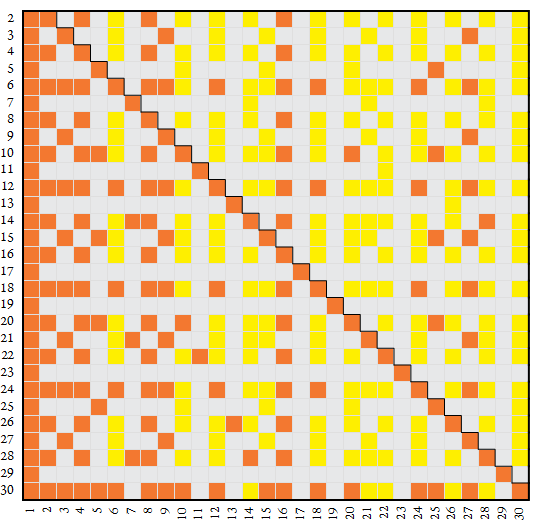
Figure 1 shows constitutive relationships between n on the vertical axis and k on the horizontal. The n-regular k (i.e., A304569(n,k) = 1) appear in orange (■), n-semicoprime k (i.e., A304572(n,k) = 1) appear in yellow (■), and n-coprime k > 1 (i.e., A054521(n,k) = 1 for k > 1) appear in light gray (■). The number k = 1 is both regular and coprime, but in the figure, k = 1 is shown in orange. Hence this is a tricolor rendition of the characteristic functions [14: A304569], [14: A304572], and [14: A054521], except k = 1 is assigned regularity.

Infinite classes pertaining to the squarefree kernel of n.

Let r be an n-regular k, s an n-semicoprime k, and t an n-coprime k. Let rad(m) [14, A007947] be the squarefree kernel of m, thus, rad(12) = 6, since 6 is the product of the distinct prime divisors of 12.

For n > 1, the number of n-regular r is infinite. There are a finite number of distinct prime divisors p | n [14, A001221], yet we can produce n-regular numbers r with no p at all (since 1 is the empty product), or any number of p with multiplicity. We can produce the n-regular n as the tensor product R of the prime power ranges p^m, with m ≥ 0; all such products k are unique and therefore we can sort them. Thus, the cardinality of R is ℵ₀. For n = 1, the only n-regular number r = 1 since 1 is the empty product; all primes are coprime to 1. To be more precise, we usually refer to R as a list, or a “flattened” version of the tensor product, ∪R. The same is true for similar structures described in this section. The analysis of these tensors is beyond the scope of this work.

For all n, the number of n-coprime t is infinite. All primes q > n are coprime to n and there may be some primes q < n also coprime to n. Since the number of primes is infinite with cardinality ℵ₀ and all nondivisor primes q are coprime to n, almost all primes are coprime to n. We can also produce n-coprime numbers t with no q at all (since 1 is the empty product), or any number of q with multiplicity. Here we see again that 1 is both regular and coprime to n. Thus, the cardinality of T is ℵ₀. For n = 1, all k are n-coprime since 1 is the empty product; all primes are coprime to 1.

For n > 1, the number of n-semicoprime s is infinite. So long as we have at least one p and at least one q as factors, we may select or repeat any p or q as additional factors to get an n-semicoprime product s. Again is S sortable since all the possible products are unique, thus S has cardinality ℵ₀. For n = 1, there are no 1-semicoprime numbers.

Numbers that have arithmetic relationship to the squarefree kernel rad(n) have the same relationship to any number with the same set of distinct prime factors of rad(n). In other words, each of the constitutive classes pertains to the distinct prime divisors p of n regardless of their multiplicity. Because of this, R, S, and T pertain to the squarefree kernel K of n.

For instance, the set of numbers R₆ = {1, 2, 3, 4, 6, 8, 9, 12, 16, 18, 24, 27, 32, 36, …} [14, A003586] are regular to 6, but also to 12, 18, 24, 36, 48, 72, etc., generally m × R_m where m = rad(n). The Hamming numbers {1, 2, 3, 4, 5, 6, 8, 9, 10, 12, 15, 16, 18, 20, …} [14, A051037] are regular in any n that has all of {2, 3, 5} as distinct prime divisors. R is the least dense of the three classes.

Likewise, we find n-semicoprime s in S_n. Examples include S₆ = {10, 14, 15, 20, 21, 22, 26, 28, 30, …} [14, A330136], S₁₄ = {6, 10, 12, 18, 20, 21, 22, 24, 26, 30, …} [14, A316991], etc.

Finally, the numbers t ≡ ±1 (mod 6) comprise T₆ = {1, 5, 7, 11, 13, 17, 19, 23, 25, …} [14, A007310], just as the numbers t ≡ ±1 or ±3 (mod 10) appear in T₁₀ = {1, 3, 7, 9, 11, 13, 17, 19, 21, …} [14, A045572].

Therefore, finding rad(n) = m, we may find n-regular r in R_m, where divisors d appear among r in the range 1..n. Likewise we find n-semicoprime s in S_m, and n-coprime t in T_m.

Generation of T_m is relatively simple once the reduced residues of m are found. We may find R_m by testing m^ε, ε ≥ 0. Computationally, one may find n-regular k via n^k mod k ≡ 0; there are at least 8 viable methodologies. The most efficient generation of R_m constructs m-regular r. Computationally, we look toward loops associated with distinct prime divisors p | m, limited by log_p w, where w is m divided by the product of the containing primes. This technique therefore has rank ω(m) but is efficient for m of reasonable magnitude. Once we have both R_m and T_m under a given bound v, S_m = V \ (R_m ∪T_m), where V = 1 ≤ k ≤ v. Finding S_m in this manner avoids intensive factorization.

Lastly, we see that the set of K-regular numbers m ∈ R_K = ∪(⊗({ p^ε : ε > 1 ∀ p | K }) ), for squarefree K such that ω(K) > 1, we have many elements m : ω(rad(m)) < ω(K). All m ∈ R_K are K-regular. We may guarantee K | m via m ∈ KR_K, and thereby deem such K-strongly regular. Setting aside the sets R_K and KR_K, we may say that k and n are strongly regular iff rad(k) = rad(n), and that k and n belong to KR_K.

Let S = rad(k) and let T = rad(n). We define k and n weakly regular iff S | T or T | S and S ≠ T, but strongly regular iff S = T. Therefore 5 and 10 are weakly regular as is any prime power p^ε | n iff n is neither squarefree nor prime power (i.e., n ∈ A126706). The numbers 12, 6, 18, and 384 are strongly regular.

The constitutive relations have fundamental applications toward the practical usage of base n, where coprimality implies purely recurrent unit fraction expansions, regularity terminating unit fraction expansions, and semicoprimality mixed recurrent unit fraction expansions [15]. There are other applications, regarding patterns in the base-n multiplication table, in certain divisibility rules, etc. These applications were covered in [16] and lie beyond the scope of this paper.

Omega multiplicity classes.

It is helpful to subdivide the composite numbers into classes according to the number of distinct prime divisors ω(m) and the multiplicity of prime power factors p^ε | m. We call numbers m that have 1 distinct prime factor (i.e., ω(m) = 1) prime powers; this includes primes p and composite prime powers p^ε such that ε > 1. The latter m ∈ [14: A246547] we shall call multus numbers since they have many copies of the same prime. We call numbers m that have only one copy of each distinct prime factor squarefree; this also includes primes p and composite squarefree numbers. The latter m ∈ [14: A120944] we shall call varius numbers since each prime factor is distinct. Finally, the rest of the composite numbers have both more than 1 distinct prime divisor (i.e., ω(m) > 1) and more than 1 copy of at least 1 distinct prime factor p (i.e., ∃ p^ε | m : ε > 1). Such m ∈ [14: A126706] we shall call tantus numbers since they have so many of both distinct prime divisors and multiplicity of at least 1 such factor. These Latin names are intended to streamline certain aspects of describing the constitutive relations between 2 numbers, since these discriminate between 1 or many each of distinct prime factors and multiplicity of at least one such factor. See [17] for more.

Hence, along with primes, there are 4 omega-multiplicity classes, where m = 1 is simply the empty product and stands outside the framework presented below. We use the function M(n) to signify the largest exponent of a prime power factor p^ε | m.

Omega-Multiplicity Diagram

	M(n) = 1	M(n) > 1
ω(n) > 1	■ multus 8, 27, 125 A246547	■ tantus 12, 75, 216 A126706
ω(n) = 1	■ prime 2, 17, 101 A40	■ varius 6, 35, 210 A120944

Constitutive counting functions.

We can create counting functions by applying a bound to k related to n and assessing how many k are regular, semicoprime, or coprime.

The Euler totient function is most inherent and well-known [14: A000010]. We might also refer to the function as the totative counting function, as it is the number of t < n coprime to n. Such numbers are called totatives or reduced residues t of n. Given the standard prime power decomposition of n:

φ(n) = n × Π (1 − 1/p)                                                          
= n ×(1 − 1/p₁) ×(1 − 1/p₂) × … × (1 − 1/p_i) [11]

We note that φ(n)/n = Π (1 − 1/p), the totient ratio, is only dependent on the distinct prime divisors p | n but not their multiplicities ε. The totient ratio is shared among numbers n that have the same squarefree kernel. For example, φ(6)/6 = φ(12)/12 = 1/3, in other words, one third of the numbers 1 ≤ k ≤ n are coprime to n. Likewise, φ(10)/10 = φ(20)/20 = 2/5, φ(2)/2 = φ(4)/4 = φ(8)/8 = φ(16)/16 = 1/2.

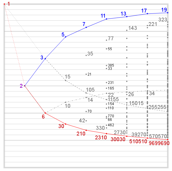
Figure 2 illustrates the totient ratio for squarefree n. The vertical axis represents the totient ratio φ(m)/m, 0 at bottom and 1 at top, while the horizontal represents the number of distinct prime divisors of squarefree m. On the chart, we can find the totient ratio for any n by finding the point representing φ(m)/m, where m is the squarefree kernel of n. [14: A307540]. The higher the totient ratio φ(n)/n, the greater the chance that an arbitrary nonzero positive integer k is coprime to n.

The reduced residue system (RRS) of n contains all the totatives t of n. For example, RRS(10) = {1, 3, 7, 9}. Given the RRS, we can determine all n-coprime numbers using congruency. A number k is coprime to n if k mod n ≡t. Any number k = ±1 (mod n) is coprime to n since 2 is the smallest prime [10]. Since the RRS is indicative of n-coprime numbers by congruence, the application of n as a bound for an n-coprime counting function makes sense.

The divisor counting function τ(n) is similarly inherent and well-known [14: A000005]. No divisor d can exceed n, thus the number of divisors is finite and a bound at n [14: A275055] makes sense regarding this special case of n-regular r. Given the standard form prime power decomposition of n:

τ(n) = Π (ε + 1)                                            
= (ε₁ + 1) × (ε₂ + 1) × … × (ε_i + 1)

The regular counting function RCF(n) is less-well known [14: A010846] and not as easy to compute [14: A275280]. The bounding of the function τ(n) to include d ≤ n is natural, since divisors cannot exceed n. It is less natural perhaps to consider the regular numbers r ≤ n, since there are an infinite number of semidivisors larger than n.

There are some interesting properties of RCF(n) that perhaps underscore a purpose for the bound. We might link the n-regular k with the proper divisors of n to create n-proper regulars ρ. We call k a proper regular number ρ with respect to n iff LCM(k, n) ≠ k. This has the effect of boiling out perfect powers of n from n-regular k, collapsing k into families ρ × n^ε for ε ≥ 0. For example, the 10-regular numbers begin as follows:

1, 2, 4, 5, 8, 10, 16, 20, 25, 32, 40, 50, 64, 80, 100, 125, 128, 160, 200, 250, 256, 320, 400, 500, 512, 625, 640, 800, 1000, 1024, 1250, 1280, 1600, 2000, 2048, 2500, 2560, 3125, 3200, 4000, 4096, 5000, 5120, 6250, 6400, 8000, 8192, 10000, …

These can be arranged into familes 1 × 10^ε, 2 × 10^ε, 4 × 10^ε, 5 × 10^ε, 8 × 10^ε, 16 × 10^ε, 25 × 10^ε, etc. and it becomes evident that we might express R₁₀ as follows:

{R₁₀∀(α ∈ N, β ∈ N, ε ≥ 0) : 2^α × 10^ε ∪ 5^β × 10^ε}

The proper regulars of n = 10 are simply any product of at least 1 or both of 2^α and 5^β that is not a perfect power 10^ε. In decimal notation, the proper regulars of 10 are any decimal regular number that has no trailing zeros. Generally, represented in base b, the proper regulars of b have no trailing zeros. It is clear the proper divisors of b are a subset of the proper regulars of b.

For base n = 12, the proper regulars are { k ∈ R₆ : 12 ∤ k} ⊂ { d | 12 : d < 12} [14: A353383]. We can construct the set by sorting { {2^2m−1, 2^m, 3^m, 2 × 3^m} : m ≥ 1 }.

For base n = 20, the proper regulars are { k ∈ R₁₀ : 20 ∤ k} ⊂ { d | 20 : d < 20} [14: A353384]. We can construct the set by sorting { {2^2m−1, 2^m, 5^m, 2 × 5^m} : m ≥ 1 }.

For base n = 60, the proper regulars are { k ∈ R₃₀ : 60 ∤ k} ⊂ { d | 60 : d < 60} [14: A353385]. (See that sequence for more information if desired.)

It is clear that, for n that is not a prime power (i.e., n ∈ A024619), we can produce an infinite sequence of proper regular k with respect to n.

For any prime power n = p^ε (i.e., n ∈ A246655), the set of proper regulars is finite: {1, p, p ^j, …, p^{(ε − 1)}} with 1 ≤ j < ε. For example, the proper regulars of 16 are simply {1, 2, 4, 8}. These numbers, followed by any number of zeros in hexadecimal notation (including no zeros) are regular to 16.

Primes n = p and perfect prime powers n = p^ε do not have semidivisors r < n. Numbers 1 ≤ k ≤ p must either divide or be coprime to p in the first case, and all regular 1 ≤ k ≤ p^ε, are divisors in the second case as they are themselves perfect prime powers p^m with 0 ≤ m ≤ ε. Of course, n itself is n-regular, and as stated, divisors, a special case of n-regular number, may not exceed n. For this reason, people have determined a motivation to create a counting function for regulars r ≤ n.

We might derive a semidivisor counting function ξ_d(n) that counts nondivisor regulars r < n:

ξ_d(n) = RCF(n) – τ(n),
   = ξ(n) − ξ_t(n)

or in terms of the OEIS:

A243822(n) = A010846(n) − A000005(n),
                    = A045763(n) − A243823(n)

The bound at n does not seem as useful as regards semidivisors but for the fact that divisors, the other class of n-regular numbers, is indeed effectively bounded at n.

Given the Euler totient function and the regular counting function, we can determine the semicoprime counting function, which we instead call the semitotative counting function ξ_t(n) [14: A243823].

ξ_t(n) = n − (RCF(n) + φ(n) − 1),
   = ξ(n) − ξ_d(n)                

or in terms of the OEIS [14]:

A243823(n) = n − (A010846(n) + A000010(n) − 1),
                  = A045763(n) − A243822(n)

The bound at n seems least useful as regards n-semicoprime s but for the fact that the bound makes at least some sense for the other two constitutive classes.

We can combine the semidivisor and semitotative counting functions to produce a “neutral counting function” that counts numbers 1 ≤ k ≤ n that are not counted by neither the divisor counting nor the Euler totient function. Indeed this is [14: A045763], which is fairly easy to calculate:

ξ(n) = n − (τ(n) + φ(n) − 1)
= ξ_d(n) + ξ_t(n)      

or in terms of the OEIS:

A045763(n) = n − (A000005(n) + A000010(n) − 1)      
= A243822(n) + A243823(n)

Since the counting functions break the constitutive classes into easily constructible subcomponents, we can thus produce the following figure.

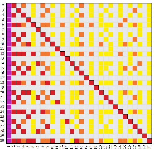
Figure 3 shows n on the vertical axis and k on the horizontal. Divisors k | n : k > 1 appear in red (■) and nondivisor n-regular k (semidivisors) appear in orange (■), n-semicoprime k appear in yellow (■), and n-coprime k > 1 appear in light gray (■). The number k = 1 is both regular and coprime and appears in purple (■).

Constitutive binary relations.

We know that k | n does not necessitate n | k; indeed k | n and n | k are both true iff k = n, since in order for one number to divide the other, the former may not exceed the latter. Similarly, n-regular k does not imply k-regular n. Indeed n-regular k and k-regular n both true iff rad(k) = rad(n), that is, if and only if k and n share the same squarefree kernel K. It is often the case that while we have n-regular k, n may have at least 1 factor q that does not divide k. We note that k ¦ n iff both k and n are composite, since prime k may only either divide or be coprime to n. Finally, k ◊ n may be n-regular as already discussed. We have commutative semicoprimality only given numbers k and n that each have factors m > 1 distinct from one another that do not divide the other number. Therefore, the only constitutive relation that is reliably commutative is coprimality; the others are conditionally commutative.

We can devise ten binary constitutive states and assign them codes so as to succinctly label a given binary relation. Since coprimality is commutative, we assign this state the code 0.

Let c(m) = −1 if k ◊ n, 0 if k | n, or 1 if k ¦ n. Similiarly, c'(m) = −1 if n ◊ k, 0 if n | k, or 1 if n ¦ k. We may define a sequence C(m) = 3×(c(m)+1) + (c'(m)+1) + 1 and thereby derive 9 possible states into which {k, n} might fall. Therefore we have ten possible states C(m) that are mutually exclusive for m > 1.

Table 2: states of constitutive binary relations between k and n:

	|	k ◊ n	k | n	k ¦ n
-------	|	-------	-------	-------
n ◊ k	|	(1)	(4)	(7)
n | k	|	(2)	(5)	(8)
n ¦ k	|	(3)	(6)	(9)

Typically we write the constitutive binary states as a circled numeral, or a numeral in parentheses (perhaps for clarity), so as to distinguish these from numbers.

States (0), (1), (5), and (9) are symmetric; (0) is the coprime state which is implicitly symmetrical, (1) the symmetrically semicoprime state, state (5) symmetrically divisible state, and (9) symmetrically semidivisible. We have already described the circumstances wherein k and n enjoy commutative states. We often experience symmetrically coprime and symmetrically semicoprime states, whereas symmetrical divisibility implies equality of k and n. Symmetrical semidivisibility is rare, since semidivisibility is completely regular, and the regular relation is the least dense of the three basic constitutive relations.

Since we say a state is neutral if it involves k neither dividing n nor coprime to n, we have completely neutral states in (1), (3), (7), and (9), which imply k and n both composite. Only k- and n-divisor states (2), (4), (5), (6), and (8) that include k | n or n | k may harbor a prime k or prime n respectively. We say that states (3) and (7) are mixed neutral, since one side is semicoprime to the other, and the other is regular to the first.

We have completely regular states in (5), (6), (8), and (9). Since state (9) is both completely regular and completely neutral, k and n must have the same squarefree kernel K and neither k nor n may be prime (see Theorem R3). States (6) and (8) are mixed regular, since one side divides the other, yet the other semidivides the first.

Asymmetrical binary relations have reverse relations. For instance, with k = 5 and n = 10, we note that 5 | 10, but 10 ◊ 5, since 2 | 10 but does not divide 5. This binary relation between 5 and 10 represents state (4). We could write “5 ④ 10” or “5 |◊ 10” for concision. We may set k = 10 and n = 5 to reverse the entire relation to obtain 10 ◊ 5 ∧ 5 | 10 which is still true, only reversed, thus, we have state (2), the reversal of state (4). This could be written “10 ⑤ 5” or “10 ◊| 5”. Surely, we may also reverse the symmetrical relations (0), (1), (5), and (9); their reverse relation is themselves.

For either k or n equal to 1, by convention, we only allow state (0). For k = n = 1, we allow state (5). The state k | n ∧ n ⊥ k implies k = 1, while its reverse, state k ⊥ n ∧ n | k, implies n = 1, but it is also true that state (0) applies to both, therefore we define 1 = k or 1 = n as having state (0).

The symmetric completely-neutral and completely-regular state (9) concerns k and n of a particular relationship that makes it a relatively rare state. The numbers k ≠ n, both composite, share the same squarefree kernel K = rad(k) = rad(n), that is, their set of distinct prime divisors are identical. The example of 12 and 18 serves to underscore this fact; both have {2, 3} as their distinct prime factor set. However, we can find k, n : rad(k) = rad(n) but k | n, e.g., 12 | 24 ∧ 24 ¦ 12, state (6), or if reversed, state (8), still completely regular. The reason why 12 ¦ 18 ∧ 18 ¦ 12 concerns the multiplicities of the distinct prime factors (see Lemma 9.2). For k = 12, we have 2² × 3, whereas n = 18 = 2 × 3². The numbers are squareful, but additionally there is another necessary quality. Therefore, the factor 2 is “rich” in 12 compared to 18, and the factor 3 is rich in 18 compared to 12; the numbers are “mutually rich” and thus we have state (9), 12 ¦¦ 18. It is clear that such numbers are strongly regular. Therefore we may select other mutually rich K-regular numbers, for example with K = 6, 72 ¦¦ 54, 96 ¦¦ 144, etc.

The K-regular k must have more multiplicity in at least 1 distinct prime factor than does K-regular n, and n must have more multiplicity in at least 1 different distinct prime factor then does k. Hence, the domain of state (9) is m ∈ A126706 [17, the “tantus” numbers] (see Corollary 9.3). This demonstrates the relative rarity of the state among arbitrary k and n.

Of course, given k = n, both composite (and of course even prime or 1), we have state (5) and not state (9) (see Lemma 9.2).

Symbolic abbreviations. We may abbreviate constitutive binary relations by placing a non-coprime symbol, ( ◊, |, or ¦ ) on the side of the number to which it pertains. For example, we may write traditional k | n in three ways to specify binary relations. For instance, 6 | 12 may be more precisely rendered as 6 |¦ 12, since 6 divides 12, but 12 semidivides 6. The tautological 6 | 6 may be more precisely written 6 || 6 for obvious reasons. And 10 | 30 may be more precisely rendered 10 |◊ 30 since though 10 divides 30, 30 is semicoprime to 10, since 3 | 30 but 3 is coprime to 10.

If we want to be clearer, we might interpose a period (full stop) between component symbols for clarity. Hence 6 || 6 might be better read as 6 |.| 6, and 6 |¦ 12 more legible as 6 |.¦ 12. Another alternative is to stick with the numerical classes. Then 6 || 6 becomes 6 (5) 6 and 6 |¦ 12 as 6 (6) 12, though encircled numerics are superior provided they are written sufficiently large, because this way parenthetic numerals aren’t deemed multiplication.

In general, constitutive binary relations are determined by the number ω(m) of distinct prime divisors p | m and the multiplicities ε of prime power factors p^ε | m of the inputs m. Hence, omega-multiplicity classification [17] is helpful in analyzing such relations. Certain relations are restricted to m of a given omega-multiplicity classification.

Table 3 summarizes the constitutive binary relations and their qualities. Examples appear in the note. For coprimality, we may consider any 2 dissimilar primes p and q. Symmetric divisibility applies only to k = n.

C	binary relation	abb.	sym.	neut.	reg.	rev.	note	domain:
----	------------------	------	------	------	------	------	------------------	------------------------------------
⓪	k ⊥ n ∧ n ⊥ k	⊥	✓			⓪	∀ p, q, p ≠ q	m ∈ ℕ
①	k ◊ n ∧ n ◊ k	◊◊	✓	✓		①	6 ◊◊ 10	m ∈ A2808
②	k ◊ n ∧ n | k	◊|				④	30 ◊| 6	k ∈ A2808 ∧ n ∈ ℕ
③	k ◊ n ∧ n ¦ k	◊¦		✓		⑦	30 ◊¦ 12	k ∈ A2808 ∧ n ∈ A126706
④	k | n ∧ n ◊ k	|◊				②	10 |◊ 30	k ∈ ℕ ∧ n ∈ A2808
⑤	k | n ∧ n | k	||	✓		✓	⑤	k || n ∴k = n	m ∈ ℕ
⑥	k | n ∧ n ¦ k	|¦			✓	⑧	6 |¦ 12	k ∈ ℕ ∧ n ∈A013929
⑦	k ¦ n ∧ n ◊ k	¦◊		✓		③	20 ¦◊ 30	k ∈A126706 ∧ n ∈ A2808
⑧	k ¦ n ∧ n | k	¦|			✓	⑥	20 ¦| 10	k ∈A013929 ∧ n ∈ ℕ
⑨	k ¦ n ∧ n ¦ k	¦¦	✓	✓	✓	⑨	12 ¦¦ 18	m ∈ A126706

Directionality and greedy solutions.

We may find interest in the difference (n − k) and the ratio n/k for divisor states ②④⑥⑧ (see Theorem D1). Thus, when the difference is positive or ratio is greater than 1, we would say that the state increases, and when the difference is negative or the ratio is a unit fraction, we would say the state decreases. If we can show that the state always increases, always decreases, or k = n, we would say the state is “directional”, otherwise we would say the state is “ambidirectional”, meaning it could increase or decrease. If we have k = n, then we say the state is “flat” or constant, but prefer the former so as to distinguish the meaning from other notions of the term “constant”.

We know that n = k ± 1 implies k ⊥ n, hence, if we are minimizing the difference (n − k), we need only increment to find a solution in state ⓪.

Because non-coprime states (outside of ⓪) occur in the cototient of both k and n, we can remark about the magnitude of these differences for each state below. For divisor states, we recognize max(k, n)/min(n, k) = m : integer m > 1.

Furthermore, we have directionality in terms of the number of distinct prime divisors, hence the difference (ω(n)−ω(k)). We might call this “omega-directionality” For mixed neutrality and mixed regularity, one term necessarily has more distinct prime factors than the other, while for symmetric semidivisorship the number of distinct prime divisors is the same on both sides. (see Lemma 24.1, 37.2, and 68.2)

For asymmetric semidivisibility, we have multiplicity-directionality, that is, for at least 1 common prime factor p^δ | k and p^ε | n such that δ ≠ ε. (See Lemma 68.3)

Finally, if we are approaching a solution to an axiom using a greedy algorithm, the difference between numbers that satisfy certain constitutive states becomes relevant. We know that we can find adjacent coprime numbers, since m ⊥ (m±1). However, k ⑨ n implies | k − n | ≥ rad(k) ≥ 6 (see Lemma 9.4).

General description of states and their reversals.

State ⓪ (⊥) — (symmetric) coprimality:

7 ⊥12, since 12 = 2² × 3 and 7 doesn’t appear among these factors. The prime 7 does not divide 12, hence it is coprime to 12. 1 ⊥ 5, since 1, the empty product, is coprime to all n. 5 ⊥127, since 5 and 127 are dissimilar primes.Generally, any 2 distinct primes p and q are coprime, any number and 1 are coprime, and 1 is coprime to itself. Except in the case 1 ⊥ 1, state ⓪ is ambidirectional because of its symmetry and the fact k and n must be distinct. The minimum difference (n − k) = ±1.

State ① ( ◊◊ ) — symmetric semicoprimality:

6 ◊ 10 and 10 ◊ 6, since 6 = 2 × 3 and 10 = 2 × 5, gcd(6, 10) = 2, and 3 ⊥ 5; both of these exceed 1. 60 ◊ 21 and 21 ◊ 60, since 60 = 2² × 3 × 5 and 21 = 3 × 7, gcd(30, 21) = 3, and 10 ⊥ 7; both of these exceed 1. State ① is symmetrical and completely neutral, hence both k and n must be composite and distinct, therefore the state is ambidirectional (see Lemma 1.1). Since symmetric semicoprimality is completely neutral, both k and n must have more than 1 distinct prime factor, hence both are not prime powers, that is, both are in in A024619 (see Lemma 1.2). The minimum difference (n − k) = ±p, where p is the least common prime factor lcpf(n, k) (See Theorem G1). Therefore if we are moving from k to n and 2 | k, then (n − k) = ±2. The state is also ambidirectional in terms of ω.

State ② ( ◊| ) and its reversal, state ④ ( |◊ ) — asymmetric semicoprimality in divisorship:

6 | 30 and 30 ◊ 6, 288 ◊ 96 and 96 | 288, etc. Primes are confined to the right hand side in state ②, and the left hand side in state ④. Because of divisibility and inherent inequality, the state is directional. If p ◊| n, then p < n, and if k |◊ p, then k > p. The state ② is also directional in terms of representing a decrease in the number of distinct prime divisors from k to n, while ④ represents the opposite (see Lemma 24.1). As a consequence of semicoprimality, the larger of k and n must not be a prime power, hence in A024619 (see Corollary 24.2).

State ③ ( ◊¦ ) and its reversal, state ⑦ ( ¦◊ ) — mixed neutrality:

12 ¦ 30 and 30 ◊ 12, 12 = 2² × 3 and 30 = 2 × 3 × 5. 126 ◊ 147 and 147 ¦ 126 since 126 = 2 × 3² × 7 and 147 = 12 = 3 × 7², etc. Generally, prime powers p^ε : ε > 1 relates to composite m : ω(m) > 1 ∧ p | m in the mode p^ε ¦◊ m ∨ m ◊¦ p^ε. These states are completely neutral hence ambidirectional, with both k and n composite. State ③ is also omega-directional, in terms of representing a decrease in the number of distinct prime divisors from k to n, while ⑦ represents the opposite. Therefore, in addition to both k and n necessarily composite, state ③ requires k : ω(k) > ω(n), while state ⑦ reverses the requirements. Semidivisibility implies rad(min(k, n)) | rad(max(k, n)) (that is, k and n are weakly regular) and the terms appear in R_{rad(max(k, n)}. Hence the difference |(n − k)| scales along with the positions of k and n in R_{rad(max(k, n)}. Furthermore, the omega-multiplicity class of the term with larger ω governs that of the term with smaller ω as consequence of semicoprimality. (See Lemmas 37.1, 37.2, and Corollary 37.3, 37.4, and 37.5)

State ⑤ ( || ) — (symmetric divisibility) equality:

5 | 5, 8 | 8, etc. This state implies equality of k and n. It is symmetrical and completely regular, but not neutral, therefore admits primes as well as composites and the number 1. Since k = n, they are strongly regular. We say this state is directional on account of implicit equality of k and n, however in a sequence of mappings, the direction is flat, neither increasing nor decreasing. State ⑤ pertains to m ∈ ℕ. (See Lemma 5.1)

State ⑥ ( |¦ ) and its reversal, state ⑧ ( ¦| ) — mixed regularity:

6 | 12 and 12 ¦ 6, 20 ¦ 10 and 10 | 20, etc. These states are completely regular and occur entirely within KR_K, since rad(k) = rad(n). The numbers k and n are strongly regular (Lemma 68.2). Primes are confined to the right side in state ⑥ and the left in state ⑧. Let p^a < p^b be distinct composite powers of the same prime p; therefore we have the relation p^a |¦ p^b. Hence, k < n that are powers p^ε : ε ≥ 1 imply k |¦ n and thus direction. Because of divisibility and inherent inequality, the state is directional. (See Lemma 68.1.) Furthermore, mixed regularity implies multiplicity directionality; there is at least 1 prime divisor p | n that has higher multiplicity than p | k in state ⑥, for ⑧, the higher multiplicity pertains to k. (See Lemma 68.3)

State ⑥ requires k ∈ ℕ and n ∈ A013929 while state ⑧ requires the reverse. Let’s examine 2 special cases. In state ⑥, k ∈ A246655 (a prime power greater than 1) implies n ∈ A246547 [17, “multus” numbers, composite prime-power]; we reverse k and n for state ⑧. In state ⑥, k ∈ A120944 [17, “varius” numbers, squarefree composite] implies n ∈ A126706 [17, “tantus” numbers]; we reverse k and n for state ⑧. We see that A013929 = { A246547 ∪ A126706}. (See Corollary 68.4)

Relations in these states with K = 6, for example, occur within A3586 = R₆. Thus, we may select certain distinct k > 1 and n > 1 : k | n in A3586 and produce states ⑥ or ⑧, depending on which number appears first. Thus we may write 3 |¦ 9, 162 ¦| 18, etc. Semidivisibility implies rad(min(k, n)) | rad(max(k, n)) and the terms appear in R_{rad(max(k, n)}. Hence the difference |(n − k)| scales along with the positions of k and n in R_{rad(max(k, n)}.

State ⑨ ( ¦¦ ) — symmetric semidivisibility:

12 ¦¦ 18, 182 ¦¦ 361, etc. This state is symmetrical, completely neutral, and completely regular, occuring within KR_K for k and n both composite and exceeding 1. Hence, k and n have the same squarefree kernel K, and are strongly regular (see Theorem 9.1). Since the state is completely neutral and symmetrical among distinct k and n, it is ambidirectional. Since we require guaranteed divisibility by prime divisors p | K, and further, disjoint differences in multiplicity of distinct p, state ⑨ requires tantus numbers (i.e., m ∈ A126706, see Lemma 9.2 and Corollary 9.3). This is to say, both k and n must have ω > 1 (more than 1 distinct prime factor, i.e., a number that is not a prime power) and at least one prime power factor p^ε must have ε > 1. The difference |(n − k)| scales along with the positions of k and n in R_K. (See Lemma 9.4, 9.5, and Corollary 9.6)

Binary relation rules.

Here are some constitutive binary relation rules, assuming unless noted the 2 numbers to compare are dissimilar, since equality implies state ⑤.

1. Prime p | m ∨ p ⊥m, hence outside coprimality and equality, primes are restricted to divisor states .
1. If m < p,
   1. m | p iff m = 1 ∨ m = p, hence in the latter case, m ⑤ p implies the reverse, yet we write the former always 1 ⓪ p or 1 |⊥ p. (The symbol |⊥implies 1 in the left position for all m in the second position.)
   2. Else m ⊥ p for 1 < m < p, hence m ⓪ p.
2. If m > p,
   1. p | m iff m ≡ 0 (mod p). If p | m ∧ ω(m) = 1 (implies m composite),
      1. p |¦ m, hence p ⑥ m ↔ m ⑧ p.
      2. Else p |.◊ m, hence p ④ m ↔ m ② p.
   2. Else p ⊥ m for m ≢ 0 (mod p).
2. Composite prime power p^ε : ε > 1 [17, “multus” numbers, m ∈ A246547].
   1. If m = p^a : 1 < a ≠ ε implies {p, m} ⊂ R_p.
      1. If a > ε, p^ε |.|| p^a, hence p^ε ⑥ m ↔ m ⑧ p^ε.
      2. Else a < ε, p^ε ¦| p^a, hence p^ε ⑧ m ↔ m ⑥ p^ε.
   2. Else if p | m : p ≠ m implies at least 1 prime q | m ∧ q ≠ p.
      1. p^ε |◊ m iff m ≡ 0 (mod p^ε), hence p^ε ④ m ↔ m ② p^ε.
      2. p^ε ¦◊ m for m ≢ 0 (mod p^ε), hence p^ε ⑦ m ↔ m ③ p^ε.
3. Completely regular k ∧ n, i.e., for K = rad(k) = rad(n), {k, n} ⊂ R_K.
   1. If k | n : k < n (implies n ≡ 0 (mod k),
      1. k |¦ n, hence k ⑥ n ↔ k ⑧ n, implies n composite.
      2. Else k ¦¦ n, hence k ⑨ n ↔ k ⑨ n, implies both k and n composite.
4. Otherwise composite k ∧ n:
   1. If k | n : k < n (implies n ≡ 0 (mod k) ∧ gcd(k, n) = k) then k |◊ n, hence k ④ n ↔ n ② k.
   2. Else if k | n^ε : ε > 1 then k ¦◊ n, hence k ⑦ n ↔ n ③ k, implies 1 < gcd(k, n) < k.
   3. Else if gcd(k, n) > 1 then k ◊◊ n, hence k ① n ↔ n ① k.
   4. Else k ⊥ n, hence k ⓪ n ↔ n ⓪ k.

Repression of states.

Suppose we devise a function {f(x), x,y ∈ Z : y : C(y) ∈ {1, 2, 3, 4, 6, 7, 8, 9}}. This function x → y forbids coprimality and equality of x and y to yield the least y satisfying the constitutive condition. For example, if x = 6, then we may select the least y such that C(y) is neither ⓪ nor ⑤, that is ¬(x ⊥ y) ∧ x ≠ y. This is tantamount to y belonging to the cototient of and distinct from x. We can rewrite the function as {f(x), x ∈ Z : (x,y) > 1 ∧ x ≠ y}.

Now suppose we devise a sequence S given a seed S(1) and obtaining distinct terms n through remapping the function f such that the previous term serves as input k for the next remapping. Indeed, we may modify the input through incrementation, etc., so as to try to obtain a permutation of the natural numbers. Such sequences place interesting constraints on constitutive binary relations and yield interesting scatterplots. Examples of such are the Yellowstone sequence [14, A098550], the EKG sequence [14, A064413], and the Olson sequence [14, A347113], to name 3. Of these, the EKG sequence is the simplest. It is simply the distinct remapping of {f(x), x,y ∈ Z : y : C(y) ∈ {1, 2, 3, 4, 6, 7, 8, 9}} with the seed {1, 2}, 1 appearing so as to render a permutation of natural numbers, but not functioning as input. The Yellowstone sequence involves 2 distinct inputs i and j and output k. The relation (i, k) > 1 requires k belonging to the RRS of j. The Olson sequence increments j but is otherwise the same as EKG.

In such sequences, the prohibition of coprimality forces primes into divisibility states. Since k | n implies k < n and therefore, sequence increase on account of a prohibited state ⑤, states ④ and ⑥ imply increase. Conversely, since n | k implies k > n and therefore, sequence decrease on account of a prohibited state ⑤, states ② and ⑧ imply decrease.

We find that the completely neutral states that are not also completely regular, i.e., states ①, ③, and ⑦, are ambidirectional. Though the symmetrically semidivisible state ⑨ does not prohibit k > n, it may be rarely seen if we are selecting the least n such that f(k) is satisfied. State ①, the symmetrically semicoprime state, represents the least order since gcd(j, k) may be as low as p prime. State ⓪ is often the commonest state in a sequence that is a remapping of f with distinct terms.

Ambidirectional states pose an obstacle against streamlining algorithms to generate distinct remapping sequences with constraint on constitutive binary relations, especially given the predominance of such states, because we cannot predict the behavior of terms in such states.

Constitutive patterns in PDRLES.

Consider a prime divisor restricted lexically earliest sequence (PDRLES) or “pearl” sequence, for example, the EKG sequence [14, A064413], wherein coprimality is prohibited between adjacent terms. The lexical axiom of LES generally prohibits equality, forcing primes into divisibility. Divisor states, ②④⑥⑧, comprise the only avenues for the entry of primes in these sequences. A more detailed study of the EKG sequence appears in [18].

The main axiom behind the EKG sequence is non-coprimalty of adjacent terms k = a(n−1) and n = a(n). Therefore if we can find a common factor between k and n and if n is the smallest such number that has never appeared in the sequence, we satisfy the axiom. If 2 | k, then it is likely that n = k + 2, and generally, if p | k, then n = k + p, etc. (See the Lagarias-Rains-Sloane paper at [14, A064413] and the nature of controlling primes). For the most part, k ① (k + p), which is the principal reason behind the central quasi-ray in scatterplot, and it is implied that this quasi-ray is completely composite. For similar reasons, symmetric semicoprimality ① is the dominant mode of all pearl sequences.

We note that semidivisibility in divisorship (state ② and its reverse, ④) characterizes primes p in the EKG sequence. Note the Lagarias-Rains-Sloane chain 2p → p → 3p is normally 2p ② p ④ 3p, for p > 3. Other states occur according to accident: for p = 2 we have 1 ⓪ 2 ⑥ 4 and p = 3 we have 6 ② 3 ⑥ 9. Therefore, state ② represents the normal input and state ④ the normal output state for primes p in the EKG sequence and other pearl sequences. We may say that the signature for primes in the EKG sequence (and many other LES) is ②④.

Multus numbers p^ε : ε > 1 (i.e., composite prime powers m ∈ A246547) enter only after many multiples mp in the EKG sequence on account of their magnitude in geometric progression. Hence the normal input state is ③, while the normal output state is ⑦, as state ① is closed to multus numbers. In the EKG sequence we have the defect of 2 ⑥ 4 ⑦ 6 ② 3 ⑥ 9 as an accident related to small numbers.

Though mixed neutrality ③⑦ is a signature of multus numbers in the EKG and other sequences, we can find the accidental occasion of singleton states. In the EKG sequence, we note a(1220..1221) = 1290 ③ 1280, first case of singleton state ③, and a(1383878..1383879) = 1417176 ⑦ 1417182, first case of singleton state ⑦. Let s = min(n, k), t = max(n, k), and S = rad(s), where s ∈ SR_S. These are the case of s + S = t such that S | t, in other words, t = (s+1)/S. Though rare, there are likely an infinite number of singleton states ③ and ⑦ in the EKG sequence,

Due to the nature of completely regular states ⑥⑧⑨, we find these rarely in pearl sequences; as n increases, their likelihood of materializing decreases. Recall that, for mixed regular state ⑥ and its inverse ⑧, we require rad(s) | rad(t), hence, with T = rad(t), s ∈R_T ∧ t ∈R_T ∧ s ≠ t. Also recall that R_T is the tensor product of the prime power ranges of K. Therefore it is clear that, when n is sufficiently large, the difference between adjacent elements in R_T becomes too large and there is always a smaller candidate to satisfy the pearl axioms. In EKG, the only completely regular state to occur is ⑥, in precisely 2 early occasions already mentioned. In Yellowstone we compare a(n−2) and a(n), since adjacent terms must be coprime. There, in addition to early ⑥, the last instance of which is a(16, 18) = 10 ⑥ 20, we have a(31, 33) = 18 ⑨ 24.

Of all constitutive states, state ⑨ is the rarest in pearl sequences, since input and output must both appear in the list KR_K where K is the squarefree kernel of both k and n. Such a list eliminates n < K, and therefore the early instances we see for ⑥⑧.

Hence, using constitutive states, we can ably analyze LES that restrict divisibility in some way.

Furthermore, we may write more restrictive pearl sequences by constraining output according to constitutive states. As an example, we identify several constitutive restrictions of the EKG (E) and Yellowstone (Y) sequences. The numbers that follow the letters represent states to which we restrict output. For example, E24 restricts the EKG axioms such that we either have state ② or ④ (in line with the signature of primes in the original EKG sequence). Restriction of an LES to ①③⑦⑨ essentially constrains the sequence to composite numbers, as does restriction to ③⑦ or just ①.

E	A064413	Y	A098550
--------	------------	--------	------------
E1	A337687	Y1	A352098
E24	A113552	Y24	A352394
E37	A353917	Y37	A354853
E2347	A353916	Y2347	A352720
E1379	A240024	Y1379	A352097

We can indeed generate sequences limited to directional states and very efficiently yield millions of terms by avoiding simple incrementation in a While loop. These sequences serve as hampered versions of the EKG, Yellowstone, or Olson variants.

Computation.

This section covers various computation schemes related to constitutive relations. Programs in Mathematica appear in the Appendix.

Testing.

The test f_T(x) for coprimality is elementary and simple; we look for (k, n) = 1.

Likewise, n-divisors k are easy to identify via n ≡ 0 (mod k) or (k, n) = k.

These functions comprise part of most computer algebra systems. For example, in Mathematica, the former is CoprimeQ[k, n] or GCD[k, n] == 1, and the latter is DivisibleQ[n, k] or Mod[n, k] == 0.

Conceptually, it is easy to write a test f_R(x) for n-regular k using n^k ≡0 (mod k) [Code R2]. We can distinguish n-semidivisor k from n-divisor k by finding n^k ≡0 (mod k) ∧ n ≠ 0 (mod k) or via n^k ≡0 (mod k) ∧ (k, n) ≠ k. Alternatively, we might use the following approach. Let the “factorization function” F(x) be such that it lists the distinct prime divisors p | x. The number k is n-regular iff F(k) ⊆ F(n) [Code R1].

The test f_S(x) for n-semicoprime k is similar to the last-mentioned test for n-regular k. The number k is n-semicoprime iff F(k) ⊃ F(n) [Code S1].We might also use the following approach:

k ◊ n ⇒ rad(k)/(rad(k), rad(n)) > 1 ∧ rad(n)/(rad(k), rad(n)) > 1 [Code S2]

If we are working with all three basic constitutive functions, it is just as well to find ¬(k ⊥ n) ∧ ¬(k || n) (here using || inclusive of k | n). Numbers k that are neither coprime to n nor n-regular are n-semicoprime.

List generation.

Let us presume a limit ℓ such that we assess the number of terms of a certain constitutive species in the range {1…ℓ}.

It is simple to generate a list T of n-coprime k < ℓ. We simply determine if k in the range 1..ℓ belong to the RRS of n, i.e., (k,n) = 1 [Code C1].

To compute the list R of n-regular k < ℓ, we can write a series of ω(n) nested loops limited by log_p ℓ/P, where P is the product of the remaining distinct prime divisors p | n, taking each p in turn, and sorting the result [Code R4]. This might sound involved but efficiently furnishes such a list. Other methods achieve a list of n-regular k < m via k++ and testing f_R(k) [Code R3]. Since the density of n-regular k is relatively sparse compared to those of n-coprime or n-semicoprime k, this approach may prove inefficient if we are aiming for a large m.

Given T and R, we efficiently generate the list S of n-semicoprime k by means of the following [Code S4]:

S = {1…m} \ (T ∪ R)

Otherwise we may also apply k++ and testing f_S(k) so as to generate the list S [Code S3].

Counting functions.

Set ℓ = n. We define a counting function (originally named a totient function but today this name evokes a function strictly related to n-coprime k) one that counts the number of 1 ≤ k ≤ ℓ. For coprimality and divisibility, ℓ = n makes sense, since n-coprime k occur within the reduced residue system of n, and all d | n imply 1 ≤ d ≤ n. Therefore, the totative counting function more commonly known as Euler’s totient φ(n) and the divisor counting function τ(n) employ the limit ℓ = n.

The limit ℓ = n is not as inherent vis-à-vis n-regular k or n-semicoprime k. Nonetheless, it is common to use ℓ = n to define a “regular counting function” RCF(n) = A010846(n) and a “semitotative counting function” ξ_t(n) = A243823(n). We may also calculate a “neutral counting function” ξ(n) = A045763(n) [Code N1] that enumerates nondivisors in the cototient of n. The keystone to all of these flavors of counting function is RCF(n), given φ(n) and τ(n), and the fact that we can extract ξ_t(n) via n − (RCF(n) + φ(n) − 1).

The regular counting function is efficiently delivered by a method related to the efficient construction of n-regular k in a series of nested loops [Code R5]. Instead of constructing k, we sum [k || n] (Iverson brackets) and arrive at RCF(n). A less efficient method achieves the same via k++ in {1..ℓ}, using the test f_R(k).

Given RCF(n), we may then arrive at the various novel counting function flavors by means of the formulas in the counting function section. [Code S5, S6].

Constitutive state function.

Finally, we might write a function C(k, n) whose output is the constitutive state number as explained in this work [Code 1].

Conclusion.

We have described three principal classes of natural numbers k regarding their relation to n. These are the n-coprime, n-semicoprime, and n-regular numbers k, for n > 1, found in an infinite class T, S, and R, respectively. The n-regular R is a superset of the finite set of divisors d | n. We have described counting functions known to Euler, φ(n), and the ancient Greeks, τ(n), but others in OEIS associated with the other flavors. The number n itself as bound that make sense for φ(n) and τ(n) and can be extrapolated to the other counting functions. We examined constitutive binary relations and states that have certain properties that pertain to composites or primes. If we restrict these states in certain recurrent mappings, we obtain certain states that imply increase or decrease in these sequences. We also examined methods of computation related to the constitutive relations, providing code examples and related integer sequences in the appendix.

Appendix:

Theorems pertaining to constitutive states:

Theorem G1: Let (k, n) = g. Numbers k and n in the cototient (i.e., g > 1) have difference | k − n | ≥ lpf(g). (k ⊔ n ⇒ | k − n | ≥ A020639( (k, n) ).)
Proof: We know that k ⊥ n : n = k ± 1 since 2 is the smallest prime. Suppose that both k and n are odd, and define odd prime q is the smallest prime that divides both. Suppose that n − k = p = 2. Therefore, k ≡ n ≡ 0 (mod q). Since q is an odd prime, p < q. We see k = n − 2 would mean that k (mod q) > 0, a contradiction. Furthermore, for all p < q, such is true, otherwise p | k ∧ p | n, contradicting the definition of q as least common prime factor of k and n. ∎

Corollary G2: Numbers k and n in the cototient (i.e., g > 1) have difference | k − n | > 1. (k ⊔ n ⇒ | k − n | > 1.)

Theorem S1: Let P = { prime p : p|k } and let Q = { prime q : q|n }. Semicoprimality k ◊ n implies | P ∩ Q | > 0. (k ◊ n ⇒ | P ∩ Q | > 0.)
Proof. The definition of semicoprimality shows 1 < (k, n), with k ≠ (k, n) ≠ n, hence semicoprimality is neither coprimality nor divisorship and pertains to composites. It is clear that we can find at least 1 common prime divisor p | k and p | n. The definition of semicoprimality further shows that there is at least one prime q | k that does not divide n, proving n-semicoprime k is nonregular to n. Therefore the intersection P ∩ Q is not null; it contains at least 1 prime, but P contains other primes that are not in Q. (Q is not restricted only to those primes in P; there may be primes that divide n that do not divide k.) ∎

Hence symmetric semicoprimality is both ambidirectional in magnitude and completely ambiguous in terms of number of distinct prime divisors ω.

Theorem S2: Let P = { prime p : p|k } and let Q = { prime q : q|n }. Asymmetric semicoprimality k ◊⊔ n implies P ⊂ Q and ω(k) > ω(n). (k ◊⊔ n ⇒ A1221(k) > A1221(n).)
Proof. We know (k, n) > 1 since k and n share at least 1 prime divisor p, yet at least 1 prime factor q | k does not divide n via definition of semicoprime. Such implies k and n both exceed 1. Given n not semicoprime to k, then we are left with n | k^ε : ε > 0 (with respect to the context of coprime, semicoprime, and regular relations being mutually exclusive outside the empty product with domain ℕ). If n | k, then n < k and P ⊂ Q, hence ω(k) > ω(n). If n does not divide k, yet some larger power of k, then though we cannot speak to the relative magnitude of k and n, we are left with P ⊂ Q, hence ω(k) > ω(n), proving the proposition. ∎

Hence asymmetric semicoprime states are omega-directional.

Theorem D1: Asymmetric divisor states imply s < t. (s | t ∧ s ≠ t ⇒ s < t.)
Proof. Divisors s | t must be such that s ≤ t, however, s = t implies that t | s as well. Therefore we are left with s | t such that 1 < (s, t) < t. Since s | t implies (s, t) = s, we see that indeed, s < t. ∎

Hence, asymmetric divisibility is directional.

Theorem R1: Semidivisor states k ¦ n imply rad(k) | rad(n). (k ¦ n ⇒ A7947(k) | A7947(n).)
Proof. The definition of k ¦ n is k | n^ε : ε > 1. If k divides some power of n but not n itself, it follows that no n-nondivisor prime q | k, else k would not divide any power of n at all. Hence k is either an empty product (1) or it is a product of prime divisors p | n. Now let P be the set of distinct prime divisors p | k and Q be the set of distinct prime divisors p | n. We see that P ⊆ Q. ∎

Corollary R2: Semidivisor states k ¦ n imply ω(k) ≥ ω(n). (k ¦ n ⇒ A1221(k) | A1221(n).)

Theorem R3: Completely regular states ⑤⑥⑧⑨ imply rad(k) = rad(n). (k || n ∨ k ¦| n ∨ k |¦ n ∨ k ¦¦ n ⇒ A7947(k) = A7947(n).)
Proof. We approach this problem in parts. There are 2 species of regular numbers; divisors k | n and nondivisors, which we denote as semidivisors or generally k ¦ n. Permuting these in binary relations we have the four mentioned in the proposition. Therefore we have 4 cases corresponding to states ⑤⑥⑧⑨, respectively, where state ⑧ is state ⑥ reversed.
State ⑤: Lemma 5.1 shows that k || n implies k = n, hence the squarefree kernels of k and n are identical.
States ⑥⑧: Theorem D1 shows that asymmetric divisibility implies min(k, n) | max(k, n), k ≠ n. Thus we can set s = min(k, n) and t = max(k, n) such that s < t. This simplifies the cases k ¦| n and k |¦ n to s |¦ t and Lemma 68.2, where the proposition is proved for that case.
State ⑨: Finally, we have the case k ¦¦ n, where the proposition is proved via Theorem 9.1.
Taken together, Lemma 5.1, Theorem D1, and Theorem 9.1 prove the assertions of the proposition. ∎

Corollary R4: Completely regular states ⑤⑥⑧⑨ imply ω(k) = ω(n). (k || n ∨ k ¦| n ∨ k |¦ n ∨ k ¦¦ n ⇒ A1221(k) = A1221(n).)

Hence completely regular states are flat in terms of number of distinct prime divisors (ω).

Lemma 1.1: Symmetric semicoprimality implies both k and n are composite. (k ◊◊ n ⇒ k ∈ A2808 ∧ n ∈ A2808.)
Proof: Let (k, n) = m. Since 1 < m < k and m < n, k belongs to the cototient of n yet neither k | n nor n | k. Since primes p must divide or be coprime to other numbers, k ◊◊ n is restricted to composite numbers. ∎

Lemma 1.2: Symmetric semicoprimality implies both ω(k) and ω(n) exceed 1. (k ◊◊ n ⇒ k ∈ A024619 ∧ n ∈ A024619.)
Proof: A number k semicoprime to n is defined as (k, n) > 1 yet there exists at least 1 prime q | k but not n. Symmetric semicoprimality implies that both k and n have some factor M > 1 that does not divide the other. Since k and n are at least divisible by some common prime p, and since each has at least 1 prime factor q not shared with the other, at least 2 prime factors are implied for both k and n. Hence both have at least 2 distinct prime divisors. ∎

Corollary 1.3: Primes and multus numbers (composite prime powers) cannot be symmetrically semicoprime.

Lemma 24.1: Let s = min(k, n) and let t = max(k, n). Semicoprimality in divisorship implies both ω(s) < ω(t) and t = ms such that integer m > 1. (s |◊ t ⇒ ω(s) < ω(t) ∧ t = ms : m > 1.)
Proof: t ◊ s implies that t is divisible by Q > 1 : (Q, s) = 1. s | t implies s < t (since s ≠ t else s | t ∧ t | s) and t = ms. ∎

Corollary 24.2: t cannot be a composite prime power. (t ∉ A246547.)

Lemma 37.1: Mixed neutrality implies both k and n are composite. (k ◊¦ n⇒k ∈ A2808 ∧ n ∈ A2808.)
Proof. We have shown k ◊ n implies composite k. n ¦ k implies composite n since 1 < (k, n) < n by definition of semidivisor n ¦ k as nondivisor regular n | k^ε : ε > 1. Hence k and n are neutral in both directions, while a prime must either divide or be coprime to another number. ∎

Lemma 37.2: Mixed neutrality is omega-directional, that is, for k ◊ n and n ¦ k, i.e., k ③ n, ω(k) > ω(n), and for k ¦ n and n ◊ k, i.e., k ⑦ n, ω(k) < ω(n). (k ◊¦ n ⇒ ω(k) > ω(n) ∧ k ¦◊ n ⇒ ω(k) < ω(n))
Proof: k ◊ n implies that k is divisible by Q > 1 : (Q, n) = 1, yet n is regular to k, meaning that n is a product of primes p | k and no prime q that does not divide k. Further, n does not divide k, yet rad(n) | rad(k), and it is clear that ω(k) > ω(n). The same can be said, reversing the relations, so that for k ¦◊ n, i.e., k ⑦ n, ω(k) < ω(n). ∎

Corollary 37.3: For k and n such that k ◊¦ n and ω(k) > ω(n), k cannot be multus. Mixed neutrality and n = p^ε implies n : p^(ε−j) | k ∧ j > 0.

Corollary 37.4: For k and n such that k ◊¦ n and ω(k) > ω(n), varius n implies either multus or tantus k.

Corollary 37.5: For k and n such that k ◊¦ n and ω(k) > ω(n), tantus n implies any composite k.

Lemma 5.1. Symmetric divisibility ⑤ implies k = n, positive integers.
Proof. Divisors k | n are such that k ≤ n. Yet we have k | n and n | k, and the only solution is that k = n, since all numbers divide themselves. ∎

Lemma 68.1. Let s = min(k, n) and let t = max(k, n). Mixed regularity ⑥⑧ implies s | t , S = T, s < t. (s |¦ t ⇒ s < t.)
Proof. Since s | t and since t does not divide s, s < t. Instead t | s^ε : ε > 1. ∎

Lemma 68.2. Let s = min(k, n) and let t = max(k, n). Let S = rad(s) and T = rad(t). Mixed regularity ⑥⑧ implies S = T and ω(s) = ω(t). (s |¦ t ⇒ A7947(s) = A7947(t) ∧ A1221(s) = A1221(t).)
Proof. We see that s | t and t | s^ε : ε > 1. Another way to state the latter is that t is a product of p | s and not any q that does not divide s. Therefore t shares some distinct prime factors p with s. In fact, s must have the same number of distinct prime factors p as does t, since s | t. Suppose prime P | s but not t. Then s would not divide t, instead s ◊ t. Now suppose prime P | t but not s. Then t | s^ε : ε > 1 is impossible, since there is no way to introduce the prime factor P in any power of s. Hence, the squarefree kernels of s and t are identical and thereby the number of distinct prime factors of both numbers is the same. ∎

Lemma 68.3. Let s = min(k, n) and let t = max(k, n). Mixed regularity ⑥⑧ implies a richness gradient between s and t such that, though ω(s) = ω(t), Ω(s) < Ω(t). (s |¦ t ⇒ A1222(s) < A1222(t).)
Proof. Consider prime power factors p^δ | s and p^ε | t. We know all primes that divide s also divide t and vice versa. In order for t not to divide s, but s | t, we must have at least 1 prime p for which δ < ε. ∎

Corollary 68.4. s |¦ t implies t is not squarefree. (s |¦ t ⇒ t ∈ A013929.)

Theorem 9.1: Let S = rad(k) and T = rad(n). Symmetric semidivisibility ⑨ implies S = T and ω(k) = ω(n). (k ¦¦ n ⇒ A7947(k) = A7947(n) ∧ A1221(k) = A1221(n).)
Proof: k ¦ n is defined as k | n^ε : ε > 1, thus, k must not be a product of primes that do not divide n, otherwise k could not divide any power of n at all. Since we also have n ¦ k, it is clear that primes p | k also divide n, hence the set of distinct prime divisors of k are those of n, and the product of the set is the same. Therefore rad(k) = rad(n). Furthermore this set has the same cardinality, hence ω(k) = ω(n). ∎

Lemma 9.2: Consider prime power factors p^δ | k and p^ε | n. Symmetric semidivisibility ⑨ implies δ ≠ ε for at least 2 distinct primes that divide both k and n.
Proof. Theorem 9.1 shows that k and n share the same squarefree kernel K, hence every prime p | k also divides n. If there were no further differences between k and n, then we would have k | n and n | k, thus k = n (state ⑤). Multiplicatively, the only way k and n differ, having the same squarefree kernel K, is if multiplicities are as follows. Let us also consider prime power factors q^α | k and q^β | n, p ≠ q. We must have α < β and δ > ε so that k does not divide n (thus state ⑥) and n does not divide k (thus state ⑧). If we had only 1 prime (say, p) such that the multiplicities pertaining to k and n were equal, we would again have asymmetric divisibility (mixed regularity). Hence, at least 2 prime power factors must have different multiplicities in k and n so as to have symmetric semidivisibility. ∎

Corollary 9.3: Symmetric semidivisibility ⑨ implies both k and n are tantus numbers. (k ¦¦ n ⇒ k ∈ A126706 ∧ n ∈ A126706.)

Lemma 9.4: Symmetric semidivisibility ⑨ implies | k − n | ≥ K. (k ¦¦ n ⇒ | k − n | ≥ K.)
Proof. The numbers k and n are strongly regular to one another, meaning that they are distinct terms in KR_K, where K is the squarefree kernel common to both k and n. Since terms in R_K are distinct, first differences exceed 0. We note that R₆ = {1, 2, 3, 4, 6, 8, 9, …} and see instances of first difference 1. Since the smallest difference in R_K for all K is 1 and given multiplication of R_K by K, it is clear that symmetric semidivisors k and n imply | k − n | ≥ K. ∎

Lemma 9.5: Symmetric semidivisibility ⑨ implies | k − n | ≥ 6. (k ¦¦ n ⇒ | k − n | ≥ 6.)
Proof. Since K is squarefree and symmetric semidivisibility is completely neutral, K is further a varius number (i.e., squarefree composite, in A120944). Since the smallest varius number is 6 and given Lemma 9.4, the smallest difference between symmetric semidivisors | k − n | = 6. ∎

Corollary 9.6. Symmetric semidivisibility k ⑨ n implies | k − n | ≥ K for min(k, n) = lpf(K) × K. (k ¦¦ n ⇒ | k − n | ≥ K : min(k, n) = lpf(K) × K.)
This corollary is handy in application of analysis of state ⑨ in the context of LES. Using a greedy approach and tracking first differences of the composite states (e.g., ①), it seems possible that we can rule out the emergence of state ⑨ once the sequence is sufficiently mature. This explains the rarity of state ⑨ in LES.

References

References are provided primarily to book sources to amplify research and your web searches in addition to the links to internet sources provided in the glossary. See the site reference list for general book sources and ISBNs. The books are generally deeper and handier to those interested in the subject, complete with exercises for broader understanding of the concepts herein and throughout this work.

[1] Hardy & Wright 2008, Chapter I, “The Series of Primes”, Section 1.3, “Prime numbers”, page 3, specifically: “Theorem 2. (The fundamental theorem of arithmetic) The standard form of n is unique; apart from rearrangement of factors, n can be expressed as a product of primes in one way only”, and the proof at Chapter II, “The Series of Primes”, Sections 2.10, “Proof of the fundamental theorem of arithmetic”, and 2.11, “Another proof of the fundamental theorem of arithmetic”, pages 25−26.

[2] Dudley 1969, Section 2, “Unique factorization”, page 18, specifically: “From the unique factorization theorem it follows that each positive integer can be written in exactly one way in the form n = p₁^e1 × p₂^e2 × … × p_k^ek where e_i ≥ 1, i = {1, 2, … k}, each p_i is a prime, and p_i ≠ p_j for i ≠ i. We called this representation the prime-power decomposition of n, and whenever we write n = p₁^e1 × p₂^e2 × … × p_k^ek it will be understood, unless specified otherwise, that all the exponents are positive and the primes are distinct”.

[3] Dudley 1969, Section 2, “Unique factorization”, page 10, specifically: “A prime is an integer that is greater than 1 and has no positive divisors other than 1 and itself”.

[4] Hardy & Wright 2008, Chapter I, “The Series of Primes”, Section 1.1, “Divisibility of integers”, pages 1–2, specifically: “An integer a is said to be divisible by another integer b, not 0, if there is a third integer c such that a = bc. If a and b are positive, c is necessarily positive. We express the fact that a is divisible by b, or b is a divisor of a, by b | a.”

[5] Hardy & Wright 2008, Chapter V, “Congruences and Residues”, Section 5.1, “Highest common divisor and least common multiple”, page 58, specifically: “If (a, b) = 1, a and b are said to be prime to one another or coprime. The numbers a, b, c, …, k are said to be coprime if every two of them are coprime. To say this is to say much more than to say that (a, b, c, …, k) = 1, which means merely that there is no number but 1 which divides all of a, b, c, …, k. We shall sometimes say ‘a and b have no common factor’ when we mean that they have no common factor greater than 1, i.e. that they are coprime.”

[6] Jones & Jones 2005, Chapter 1, “Divisibility”, Section 1.1, “Divisors”, page 10, specifically: “Definition: Two integers a and b are coprime (or relatively prime) if gcd(a, b) = 1 … More generally, a set of integers a₁, a₂, … are coprime if gcd(a₁, a₂, …) = 1, and they are mutually coprime if gcd(ai, aj) = 1 whenever i ≠ j. If they are mutually coprime then they are coprime (since gcd(a₁, a₂, …) | gcd(a₁, a₂)), but the converse is false.”

[7] Ronald Graham, Donald Knuth, and Oren Patashnik, Concrete Mathematics, Addison-Wesley Professional, 2nd ed., 1994. See p. 115: When gcd(m, n) = 1, the integers m and n have no prime factors in common and we way that they’re relatively prime. This concept is so important in practice, we ought to have a special notation for it; but alas, number theorists haven’t agreed on a very good one yet. Therefore we cry: Hear us, O Mathematicians of the World! Let us not wait any longer! We can make many formulas clearer by adopting a new notation now! Let us agree to write ‘m ⊥ n’, and to say “m is prime to n,” if m and n are relatively prime. “Like perpendicular lines don’t have a common direction, perpendicular numbers don’t have common factors.”

[8] Ore 1948, Chapter 4, “Prime Numbers”, page 50, specifically: “Lemma 4-1. A prime p is either relatively prime to a number or divides it” and ensuing proof.

[9] LeVeque 1962, Chapter 2, “The Euclidean Algorithm and Its Consequences”, Section 2−2, “The Euclidean algorithm and greatest common divisor”, page 24, specifically: “(e) if a given integer is relatively prime to each of several others, it is relatively prime to their product.” and the ensuing example.

[10] Ore 1948, Chapter 13, “Theory of Decimal Expansions”, page 316, specifically: “In general, let us say that a number is regular with respect to some base number b when it can be expanded in the corresponding number system with a finite number of negative powers of b. … one concludes that the regular numbers are the fractions r = p/q, where q contains no other prime factors other than those that divide b.”

[11] Eric Weisstein, Mathworld, Regular number.

[12] Wikipedia, Regular number.

[14] Sloane, Neil, The On-Line Encyclopedia of Integer Sequences, Retrieved November 2021.

[15] Hardy & Wright 2008, Chapter IX, “The Representation of Numbers by Decimals”, Section 9.6.*

[16] Michael De Vlieger, Neutral Numbers, 2011.

[17] Michael De Vlieger, Omega Multiplicity Classes, Sequence Analysis, 2022.

[18] Michael De Vlieger, Constitutive Analysis of the EKG Sequence, Sequence Analysis, 2021.

* Note: there is an error in Theorem 136 regarding the number of digits in a terminating fraction: the counterexample is the base-16 representation of 1/8 = .4 hexadecimally: a single terminating digit. By the Theorem as published, one is led to think that, any expansion of n-regular fractions x/r for r | n^ε with ε > 0 will terminate after something other than ε digits. Suppose n = 16, r = 8, and x = 1. Then, since 8 = 2³ and max(3) = 3, we would have 3 digits after the radix point, which is clearly contradicted by hexadecimal 1/8 = .4. We recognize that the number of digits a terminating fraction 1/k has in base n is the richness ε of n-regular k.

(Back to top ↑)

Code 1: Constitutive state function C(n, k):

conState[j_, k_] :=
  Which[
    j == k, 5,
    GCD[j, k] == 1, 0,
    True,
      1 + FromDigits[Map[
        Which[
          Mod[##] == 0, 1,
          PowerMod[#1, #2, #2] == 0, 2,
          True, 0] & @@ # &,
        Permutations[{k, j}] ], 3] ]

Code C1: Generate n-coprime k within the range 1…ℓ:

coprimeQ[n_Integer, lim_Integer] := Block[{k, r}, k = Floor[lim/n];
  r = Select[Range[n - 1], CoprimeQ[n, #] &];
  Join[Flatten@ Array[n # + r &, k, 0],
    k n + TakeWhile[r, # <= lim - k n &]]];

Code N1: Generate the neutral counting function ξ(n) = n − (τ(n) + φ(n) − 1) [14: A045763]:

a045763[n_] := n - (DivisorSigma[0, n] + EulerPhi[n] - 1)];

Code R1: Test if k is regular to n (method 1):

regularQ[k_Integer, n_Integer] := Or[Abs@ k == 1,
  SubsetQ[FactorInteger[n][[All, 1]], FactorInteger[k][[All, 1]]]]];

Code R2: Test if k is regular to n (more efficient method 2):

regularQ[m_Integer, n_Integer] := PowerMod[n, m, m] == 0]]

Code R3: Generate n-regular k within the range 1…ℓ via iteration on k and testing:

With[{n = 12, lim = 2^20}, Select[Range[lim], regularQ[#, n] &]]

Code R4: Efficiently generate n-regular k within the range 1…ℓ for large datasets:

Note: this function writes a series of loops and then executes them via ToExpression.

regulars[n_, m_ : 0] :=
  Block[{w , lim = If[m <= 0, n, m]},
    Function[w,
    Sort@ ToExpression@
    StringJoin["Block[{n = ", ToString@ lim, "}, Flatten@ Table[",
    StringJoin@
      Riffle[Map[ToString@ #1 <> "^" <> ToString@ #2 & @@ # &, w], " * "],
        ", ", Most@ Flatten@ Map[{#, ", "} &, #], "]]"] &@
    MapIndexed[Function[p,
      StringJoin["{", ToString@ Last@ p, ", 0, Log[",
      ToString@ First@ p, ", n/(",
      ToString@ InputForm[
        Times @@ Map[Power @@ # &, Take[w, First@ #2 - 1]]],
        ")]}"]]@ w[[First@ #2]] &, w]]@
      Map[{#, ToExpression["p" <> ToString@ PrimePi@ #]} &, #[[All, 1]] ] &@
        FactorInteger@ n];

Example of the executable for R₂₁₀ in the range 1..2²⁰:

Block[{n = 2^20}, Flatten@
  Table[2^p1 * 3^p2 * 5^p3 * 7^p4,
    {p1, 0, Log[2, n/(1)]},
    {p2, 0, Log[3, n/(2^p1)]},
    {p3, 0, Log[5, n/(2^p1*3^p2)]},
    {p4, 0, Log[7, n/(2^p1*3^p2*5^p3)]}]

Generation of R₂₁₀ in the range 1..2¹⁰⁰ takes less than 5 seconds*.

Code R5: Efficiently calculate RCF(n) [14: A010846]:

Note: this function works similar to Code R4 above. It generates RCF(P(8)) = A010846(A2110(8)) = 19985 in 1 s*, and RCF(P(15)) = A010846(A2110(15)) = 440396221 in 7:52:30 hours*. We estimate it will take 34 hours to find RCF(P(16)).

rcf[n_] := Function[w,
  ToExpression@
    StringJoin["Block[{n = ", ToString@ n, ", k = 0}, Table[k++, ",
      Most@ Flatten@ Map[{#, ", "} &, #], "]; k]"] &@
        MapIndexed[Function[p, StringJoin["{", ToString@ Last@ p, ", 0, Log[",
          ToString@ First@ p, ", n/(",
        ToString@ InputForm[
          Times @@ Map[Power @@ # &, Take[w, First@ #2 - 1]]],
            ")]}"]]@ w[[First@ #2]] &, w]
            ]@ Map[{#, ToExpression["p" <> ToString@ PrimePi@ #]} &,
            FactorInteger[n][[All, 1]]]

Code S1: Test if k is semicoprime to n (method 1):

semicoprimeQ[m_Integer, n_Integer] :=
  Count[#, _?(Mod[n, #] == 0 &)] < Length[#] && 1 < GCD[m, n] < m &@
    FactorInteger[m][[All, 1]]

Code S2: Test if k is semicoprime to n (method 2):

semicoprimeQ[m_Integer, n_Integer] :=
  If[GCD[m, n] == 1, False,
    Function[{j, k}, FreeQ[{#1, #2}, 1] & @@ ({j, k}/GCD[j, k])] @@
      Map[Times @@ FactorInteger[#][[All, 1]] &, {m, n}]]

Code S3: Generate n-semicoprime k within the range 1…ℓ via iteration on k and testing:

With[{n = 30, lim = 2^20}, Select[Range[lim], semicoprimeQ[#, n] &]]

Code S4: Generate n-semicoprime k via S_rad(n) = (1…ℓ) \ (R_rad(n) ∪ T_rad(n)). If we use Code R2, this is achieved in 1.75 s vs. 8.5 s*.

With[{n = 30, lim = 2^20}, Select[Range[lim], Nor[regularQ[#, n], CoprimeQ[#, n]] &]]

Code S5: Generate the semitotative counting function ξ_t(n) [14: A243823]:

With[{n = 210}, Count[Range[n], _?(semicoprimeQ[#, n] &)]]

Code S6: Generate the semitotative counting function ξ_t(n) via n − (RCF(n) + φ(n) − 1):

With[{n = 30, lim = 2^20}, n - (rcf[n] + EulerPhi[n] - 1)]

* These computation times pertain to an Intel® Xeon® 8-core E-2286M CPU at 2.40 GHz each, with 32 Gb RAM in a 64-bit Windows 10 environment. The computation of RCF(P(15)) was conducted in 2016 on an Intel® Xeon® 4-core E3-1535M v5 CPU at 2.90 GHz each, 32 Gb RAM in Windows 7. Computation time of course will vary based on hardware and software environments; the times are given here as a reference gauge of efficiency.

Concerns OEIS sequences:

A000005: The divisor counting function τ(n).
A000010: The Euler totient function φ(n).
A000040: The primes.
A000961: Prime powers.
A002808: The composites, { ℕ \ ({1} ∪ A40) }.
A003586: Numbers k regular to n = 6; R₆.
A005117: Squarefree numbers.
A007310: Numbers k coprime to n = 6; T₆, t ≡ ±1 (mod 6).
A007947: Squarefree kernel rad(n).
A010846: The regular counting function RCF(n) = τ(n) + ξ_d(n).
A013929: Non-squarefree numbers { ℕ \ A5117 } = { A246547 ∪ A126706}.
A024619: Numbers that are not prime powers { ℕ \ A961 } = { A120944 ∪ A126706 }.
A045572: Numbers k coprime to n = 10; T₁₀, t ≡ ±1 or ±3 (mod 10).
A045763: The neutral counting function ξ(n) = n − (τ(n) + φ(n) − 1).
A051037: Numbers k regular to n = 60; R₆₀.
A054521: Characteristic function of n-coprime k.
A064413: EKG sequence: least-distinct-y remapping of {f(x), x ∈ Z : (x,y) > 1 ∧ x ≠ y}, seed 1.
A098550: Yellowstone sequence: least-distinct sequence with (i, k) > 2, (j, k) = 1, {i, j, k} the latest 3 terms, seed {1, 2}.
A120944: Squarefree composites (varius numbers) { A5117 \ A40 }.
A126706: Numbers neither squarefree nor composite (tantus numbers) { ℕ \ (A961 ∪ A5117) } = { A012929 ∪ A24619 }.
A243822: The semidivisor counting function ξ_d(n).
A243823: The semitotative counting function ξ_t(n).
A246547: Prime powers that are composite (multus numbers) { p^ε : ε > 0 } = { A246655 \ A40 }.
A246655: Prime powers { p^ε : ε > 0 } = { A961 \ {1} }.
A275055: Irregular triangle read by rows listing d | n in order of appearance in a matrix of products that arranges prime power factors p^ε | n along independent axes.
A275280: Irregular triangle listing n-regular m that have prime divisors p | n and no other prime factor q in order of appearance in a matrix of products that arranges prime power factors p^ε | n along independent axes.
A304569: Characteristic function of n-regular k.
A304572: Characteristic function of n-semicoprime k.
A307540: Irregular triangle T(n,k) such that squarefree m with gpf(m) = prime(n) in each row are arranged according to increasing values of φ(m)/m.
A316991: Numbers k semicoprime to n = 14; S₁₄.
A330136: Numbers k semicoprime to n = 6; S₆.
A347113: Olson sequence: least-distinct-y remapping of {f(x), x ∈ Z : (x,y) > 1 ∧ x ≠ y}, seed 1, x = a(n−1)+1

Outline.

Click on a topic to visit it.

Abstract.
A. Introduction.
   Primes and constitutive relationships.
      Coprime.
   The number 1.
   Composites and constitutive relationships.
      Regular, divisor, semidivisor, semicoprime, semitotative, neutral.
B. Infinite classes pertaining to the squarefree root of n.
C. Constitutive counting functions.
   Euler totient function and totient ratio.
   Regular counting function.
      Divisor counting function.
      Semidivisor counting function.
   Semitotative counting function.
   Neutral counting function.
D. Constitutive binary relations.
   States.
    Symmetrical, completely neutral, completely regular, reverse relation.
   Repression of states.
      Directional states.
      Ambidirectional states.
E. Computation.
   Testing.
   List generation.
   Counting functions.
F. Appendix.
   References.
   Code.
   Concerns OEIS sequences.

Document Revision Record.

Note: My consideration of constitutive states began with a comment my paternal Aunt (Mary) Katherine Nuzzo made in passing during an Easter 1982 family gathering at 5126 Drummond Place, Chicago (the home of my grandparents), regarding composite numbers. I was age 11. I had asserted, given an earlier admonition by the same aunt, that I preferred composite numbers because of divisibility properties, specifically, those of the number 12. My aunt had suggested 12 was a better base than 16 sometime during Christmas 1981, given my recent affection for that base, on account of expansion of the natural fractions (1/2, 1/3, 2/3, 1/4, and 3/4). During Easter, she suggested primes were easier to work with because they had simpler binary relations [8] (she did not use that phrase). Aunt Katherine suggested that composites had complex binary relations. Because she never explained what she meant, the question burned in my mind for decades.

This paper is the result of 4 decades of thought regarding the question. The notion of binary relations among composite numbers is perhaps originally my aunt’s concept; it may be that indeed she first considered it on account of some teacher of hers, though she was brilliant. She had corrected mathematics textbooks in Chicago when still a student. Ultimately, this paper is a Christmas present from Aunt Katherine and I owe her much thanks, though she has passed. (I have dedicated other work in her honor.)

This work is dedicated to Mrs. Betty Svitek, junior high mathematics teacher at Holy Family School in Joliet, IL in the 1970s and 1980s. She had encouraged me through mathematics enrichment. Therefore this work is done in gratitude for her teaching and encouragement. Mrs. Svitek passed away in the nineties.

The constitutive states described in this paper should be called “Svitek states” in her honor. Therefore, constitutive state ① is called, “Svitek-1”, and a constitutive state function should be called the Svitek function, etc. The term “De Vlieger states”, etc., if ever considered, should never be used, instead these should be named for Mrs. Svitek.

Document Revision Record.

2021 1122 1000 Draft.
2021 1129 2130 Final.
2022 0523 2215 Minor edits.
2022 1209 1000 Edits and errata corrections.
2022 1210 0930 Connect notion of omega-multiplicity classes, correct typos.
2022 1212 1130 Addition of examples of constitutive states in LES, differences and ratios in states.
2022 1215 1030 Addition of lemmas, theorems, and corollaries; additional definitions.