The “Idaho” Sequence (A347284)
A sequence by David Sycamore (see Afterword).
Written by Michael Thomas De Vlieger, St. Louis, Missouri, 2021 0106.
Abstract.
We examine an integer sequence that constructs a number m of a given prime shape starting with prime(1)n = 2n, and thereafter, subsequent prime power factors prime( j)k = pjk where k is the greatest exponent such that pjk < p(j − 1)k(j − 1). [1] The sequence is nicknamed “Idaho” on account of the prime shape of its terms m.
The sequence has interesting properties, namely, its relationship to the Chernoff sequence, sums of first differences among the multiplicities of the prime power factors and of the prime factor factors themselves. Because of special properties of numbers in this sequence, we may compactify the large numbers in this sequence in bitmap form.
Introduction.
Let a(n) = A347284(n) be a product of prime powers pjej where pj is the j-th prime and 0 < ej = ⌊log(p(j− 1))/log(pj)⌋, beginning with 2n. [1]
In other words, a(n) = p1e1 × p2e2 × … pℓeℓ where e1 = n and ℓ is the maximum possible number of consecutive prime divisors p subject to a condition on the exponents which requires that the exponent ej > 0 is the greatest possible integer for which pjej < p(j − 1)e(j − 1) for all j ≤ ℓ. (The exponents e are stored in row n of A347285, and the power factors pe in row n of A347288.) We observe that ℓ = ω(a(n)) = A089576(n), where ω(n) = A1221(n), the number of distinct prime divisors p | n.
The sequence begins:
1, 2, 12, 24, 720, 151200, 302400, 1814400, 4191264000, 8382528000, 251727315840000, 503454631680000, 3020727790080000, 1542111744113740800000, 3084223488227481600000, 92526704646824448000000, 555160227880946688000000, 1110320455761893376000000, 10769764221549079560253440000000, 21539528443098159120506880000000, 4523300973050613415306444800000000, ...
See this list of (n, a(n)) with 1 ≤ n ≤ 145, limited by the OEIS 1000-decimal-digit threshold. Code 1 produces the sequence.
Examples:
a(0) = 1 by definition.
a(1) = 21 = 2, since there is no integer e > 0 such that 1 < 3e < 2.
a(2) = 22 × 31 = 12; 4 > 3, and there is no integer e > 0 such that 1 < 5e < 3.
a(3) = 23 × 31 = 24; 8 > 3, and there is no integer e > 0 such that 1 < 5e < 3.
a(4) = 24 × 32 × 51 = 720; 16 > 9 > 5, and there is no integer e > 0 such that 1 < 7e < 5.
a(5) = 25 × 33 × 52 × 71 = 151200, etc.
The following basic facts become clear:
1. The sequence a(n) ⊂ A025487 ⊂ A055932, that is, all terms m are products of primorials P in A2110, which are themselves products of a contiguous set of the smallest primes. This is a consequence of the definition of the sequence.
No primes pj for 1 ≤ j ≤ ℓ have e = 0 with the exception of a(0) = 20.
2. The largest primorial divisor P(ℓ) = A2110(ω(m)) = A2110(A1221(m)) | m.
3. The first prime’s power divisor is 2n, therefore, for n > 0, all terms are even.
4. The greatest prime divisor pℓ has multiplicity eℓ = 1.
5. The primes p are distinct, thus all multiplicities e are distinct as a consequence of the multiplicity condition.
6. As a corollary to (5) above, for 1 ≤ j ≤ ℓ, the multiplicity ej ≥ ℓ − j + 1.
7.
Let S be the sum of the absolute values of the first differences of the multiplicities of the prime divisors of a(n). For all n > 0, n − S = 1.
8. Let T be the sum of the first differences of the prime powers pe arranged in order of p. The sum 2n − T − pℓ = 0 for n > 0.
9. a(k) | a(n) for 0
≤ k ≤ n.
10. The numbers q = a(n+1)/a(n) are primorials, i.e., in A2110.
The “prime shape” of m.
A few definitions may aid in our analysis of this sequence.
Multiplicity notation is a handy resource that we shall define here to facilitate the discussion and examination of the large numbers that appear in a(n) and other sequences. For n = Product_(pie_i), write ei in the π(p)-th place, starting with the smallest p. Therefore, for n = 504 = 2³ × 3² × 7, we would write M(504) = “3.2.0.1”, delimiting the multiplicities with a period (full stop), and using zeros as placeholders for primes that do not appear in standard form prime decomposition of n. We may write any number of zeros after the last term in the string, since, for any nondivisor q, n = n × q0. We only need to note zeros at indices between those of primes p | n so as to maintain place value. Otherwise, it is optional to note q0 for q > pmax, since q0 is multiplicatively idempotent.
We can produce a multiplicity diagram D of m that is a histogram of the multiplicities ej at position j for prime pj | m.
Figure 1 consists of multiplicity diagrams D(a(n)) for 1 ≤ n ≤ 13:
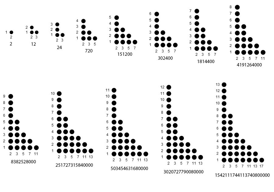
Prime shape.
In this work, the term “prime shape” refers to the arrangement of primes shown in the multiplicity diagram D(m). The term “prime shape” derives from studies of the multiplicity diagrams pertaining to the highly composite numbers (HCNs, A2182), where many have noted that the prime power divisors piei of terms in that sister subset of A025487 feature weakly decreasing exponents as i increases. Further, the prime shapes of HCNs include a long tail of largest prime divisors of multiplicity 1, and there is no prohibition for repeated multiplicities. The multiplicity diagram of the HCNs is skewed right as are those of this sequence. The HCNs m > 1 generally have the greatest exponent e1 ≤ ω(m) especially for large m. In this sequence, for n > 2, e1 > ω(m).
Figure 2 shows multiplicity diagrams of highly composite and superabundant numbers for comparison to those of terms in a(n). Here, we highlight the greatest primorial divisor P(ω(m)) | m in either A2182 or A4394, accentuating the “long tail” of large prime divisors.
This sequence is dubbed the “Idaho” sequence since the prime shape resembles that American state’s borders. We observe the multiplicity of falling away from e1 rather precipitously so as to intercept the line of slope −1 struck from the largest prime. This is to say that, for pj | m in this sequence, with 1 ≤ j ≤ ℓ, the multiplicity ej ≥ ℓ − j + 1. Here we overlay a(18) over the shape of the US state of Idaho.
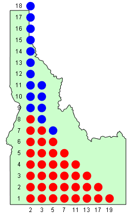
This concept also hearkens the notion of a(n) as neatly divisible by a Chernoff divisor shown in red in the diagram. This neat divisibility induces consideration of a(n) as a multiple of a specially-ordered series of indistinct primorials, evidenced by the fact that the Chernoff quotient (shown in blue) is also a product of primorials.
Basic parameters of a(n).
There are several basic parameters of a(n).
Length and width of D(a(n)).
We know that the terms a(n) for n > 0 are even since the least prime factor (2) has multiplicity n. We also know that for n > 2, ℓ = ω(a(n)) > n.
If n is thus the height of D, then ℓ represents its breadth. Hence we can obtain an auxiliary sequence L(n) = ω(a(n)) = A089576(n). This sequence begins:
0, 1, 2, 2, 3, 4, 4, 4, 5, 5, 6, 6, 6, 7, 7, 7, 7, 7, 8, 8, 8, 8, 8, 9, 10, 10, 10, 11, 11, 11, 11, 11, 12, 12, 12, 13, 13, 13, 13, 14, 15, 15, 15, 15, 15, 15, 15, 15, 15, 15, 16, 16, 16, 17, 18, 18, 18, 18, 18, 18, 18, 18, 19, 19, 19, 19, 19, 20, 20, 20, 21, 21, 21, 22, 22, 22, 22, 22, 22, 22, 22, 22, 22, 22, 22, 23, 23, 23, 23, 24, 24, 24, 24, 24, 25, 25, 25, 25, 25, 26, 27, 27, 27, 27, 28, 29, 29, 29, 29, 29, 29, 29, 29, 29, 29, 30, 30, 30, 30, 30, 30, ...
(See this list of (n, L(n)) with 1 ≤ n ≤ 104)
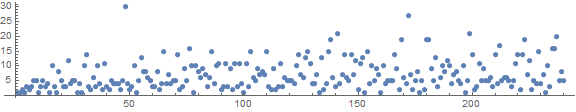
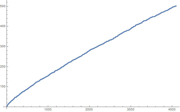
Figure 3 is a plot of L(n) for 1 ≤ n ≤ 240.
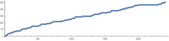
The sequence L(n) increments or remains the same as n increases. Therefore we might take the first differences d(n) (or see this list of (n, d(n)) with 1 ≤ n ≤ 104):
1, 1, 0, 1, 1, 0, 0, 1, 0, 1, 0, 0, 1, 0, 0, 0, 0, 1, 0, 0, 0, 0, 1, 1, 0, 0, 1, 0, 0, 0, 0, 1, 0, 0, 1, 0, 0, 0, 1, 1, 0, 0, 0, 0, 0, 0, 0, 0, 0, 1, 0, 0, 1, 1, 0, 0, 0, 0, 0, 0, 0, 1, 0, 0, 0, 0, 1, 0, 0, 1, 0, 0, 1, 0, 0, 0, 0, 0, 0, 0, 0, 0, 0, 0, 1, 0, 0, 0, 1, 0, 0, 0, 0, 1, 0, 0, 0, 0, 1, 1, 0, 0, 0, 1, 1, 0, 0, 0, 0, 0, 0, 0, 0, 0, 1, 0, 0, 0, 0, ...
The sequence d(n) thereby registers when L(n) changes via the value 1, or remains the same via the value 0. The position of 1s in this sequence we list in the sequence w = A347355, representing those n > 0 where ℓ = ω(a(n)) increments. When n is small it seems that 1s dominate d, but we see that ω(a(216)) = 5587. The sequence w begins (see this list of (n, w(n)) with 0 ≤ n ≤ 5587):
1, 2, 4, 5, 8, 10, 13, 18, 23, 24, 27, 32, 35, 39, 40, 50, 53, 54, 62, 67, 70, 73, 85, 89, 94, 99, 100, 104, 105, 115, 129, 132, 134, 140, 143, 153, 157, 159, 170, 173, 175, 180, 184, 188, 192, 194, 199, 229, 233, 235, 238, 248, 249, 254, 267, 275, 283, 289, 294, 297, 300, ...
A means of compressing the list L(n) of ω(a(n)), citing that ℓ(n) either stays the same or increments, is through taking run lengths of the same values and storing these in r(n) (see this list of (n, r(n)) with 0 ≤ n ≤ 5587). This is tantamount to the first differences of w:
1, 1, 2, 1, 3, 2, 3, 5, 5, 1, 3, 5, 3, 4, 1, 10, 3, 1, 8, 5, 3, 3, 12, 4, 5, 5, 1, 4, 1, 10, 14, 3, 2, 6, 3, 10, 4, 2, 11, 3, 2, 5, 4, 4, 4, 2, 5, 30, 4, 2, 3, 10, 1, 5, 13, 8, 8, 6, 5, 3, 3, 8, 2, 4, 15, 4, 7, 4, 5, 5, 14, 2, 3, 9, 5, 16, 10, 1, 10, 8, 6, 9, 7, 3, 6, 15, 4, 10, 11, 2, 3, 11, 3, 9, 2, 11, 3, 11, 4, 1, 11, 3, 15, 6, 5, 9, 7, 8, 7, 15, 3, 2, 9, ...
This list shows that certain ℓ in L(n) prove “strong”, for instance, ℓ = 47 subtending for 2n with 199 ≤ n ≤ 229.
Figure 4 is a plot of r(n) for 1 ≤ n ≤ 240.
We note the conspicuous “outlier” point r(47) = 30.
Table 1 lists the records R in r(n), the value ℓ in L(n) associated with the record, and the terms m in a(n) for n1 ≤ n ≤ n2 to which R pertains.
R ℓ n_1 n_2
-------------------------
1 0 0 1
2 2 2 4
3 4 5 8
5 7 13 18
10 15 40 50
12 22 73 85
14 30 115 129
30 47 199 229
40 429 3321 3361
44 448 3529 3573
45 1065 9800 9845
50 1375 13252 13302
59 1737 17403 17462
69 2044 20912 20981
70 4897 56566 56636
...
The Idaho sequence as a series of divisors of all succeeding terms.
We noted that the numbers m that precede a(n) in this sequence divide a(n), i.e., a(k) | a(n) for 0 ≤ k ≤ n. This follows from the definition of the sequence that has each prime power not to exceed the previous-generated prime power, beginning with 2n.
If p(j − 1)e(j − 1) increases via the iteration of e(j − 1) , pjej may or may not increase (by iteration of ej), while no change in the preceding prime power factor means the subsequent prime power factors may change. Thus, change imparted by the incrementation of 2n as n increments telegraphs for some distance, like an avalanche from a lofty peak, rolling down the side of the multiplicity diagram. When ℓ increments (i.e, when we have d(n) = 1), we have an “avalanche” that broadens the base of the diagram.
Therefore the quotients q = a(n+1)/a(n) are primorials, i.e., in A2110.
The sequence q(n) = A347354(n) of the indices of the primorial quotients a(n+1)/a(n) begins (See a table of (n, q(n)) for 1 ≤ n ≤ 216):
1, 2, 1, 3, 4, 1, 2, 5, 1, 6, 1, 2, 7, 1, 3, 2, 1, 8, 1, 4, 2, 1, 9, 10, 1, 2, 11, 1, 3, 1, 2, 12, 1, 4, 13, 1, 2, 1, 14, 15, 1, 2, 3, 1, 6, 2, 1, 4, 1, 16, 2, 1, 17, 18, 1, 2, 1, 3, 5, 1, 2, 19, 1, 4, 2, 1, 20, 1, 3, 21, 1, 2, 22, 1, 9, 1, 2, 4, 1, 8, 2, 1, 3, 1, ...
For d(n) = 1, q(n) = L(n).
The sequence q(n) serves as a more compact kernel of this sequence, since:
a(n) = Product_{k=1..n} P(q(k)).
or in terms of the OEIS:
A347284(n) = Product_{k=1..n} A2110(A347354(k)).
Indeed, the conjugate of reverse-sorting the terms q(n) for 1 ≤ k ≤ n reconstructs the multiplicities ej for 1 ≤ j ≤ ℓ, since q = a(n+1)/a(n) can be rewritten a(n+1) = q × a(n). Thus, q(n) serves as an unsorted list of indices of all primorials P(q(k)) for 1 ≤ k ≤ n that produce a(n).
Figure 5 is an animation that overlays the mutliplicity diagram D(a(n)) over that of the ensuing D(a(n+1) for 0 ≤ n ≤ 35. We can use the exponent of the leftmost prime 2 as an index:

Figure 5 accentuates the “avalanche” and conditional incrementation effect that illustrates why a(n+1)/a(n) is a primorial.
We can rewrite a(k) | a(n) for 0
≤ k ≤ n as a(n) = Product{k=1..n} A2110(q(k)). This construction of a(n) is relevant toward compactification of the large numbers in a(n) analogous to the application of OEIS A705 to furnish the superior highly composite numbers A2201, which we cover below.
The greatest Chernoff divisor ч(ω(m)) | m.
Let ч(n) = A6939(n) be the n-th Chernoff number:
ч(n) = Product_{k = 1…n} prime(k)(n − k + 1).
Therefore the sequence begins:
1, 2, 12, 360, 75600, 174636000, 5244319080000, 2677277333530800000, 25968760179275365452000000, 5793445238736255798985527240000000, ...
Code 2 generates the Chernoff numbers. (Note that the Cyrillic letter ч is a convention in this paper, not generally representative of Chernoff numbers).
The prime shape of the Chernoff numbers ч(n) is a right isosceles triangle or half-square of side length n cut in half at diametrically opposed corners. Hence, ω(ч(n)) = n and the exponent of 2 is also n. The Chernoff numbers share the property that ч(k) | ч(n) for 1 ≤ k ≤ n, however, ч(n+1)/ч(n) = P(n+1) = A2110(n+1).
Let’s return to consideration of the least multiplicity ej ≥ ℓ − j + 1 for 1 ≤ j ≤ ℓ for m in a(n). If we produce a number conforming to the least multiplicities, we have Product_{j = 1…ℓ} prime(j)(ℓ − j + 1) = ч(ℓ).
Since ℓ = ω(a(n)), we see that the greatest Chernoff divisor ч(ℓ) = ч(ω(a(n))) | a(n) is significant when we regard the prime decomposition of a(n). Through m/ч(ℓ) = k, we neutralize the largest prime power factors of m and obtain a relatively small k. Thus, we derive a sequence s(n) = ч(ω(a(n))). The sequence s(n) begins:
1, 2, 12, 12, 360, 75600, 75600, 75600, 174636000, 174636000, 5244319080000, 5244319080000, 5244319080000, 2677277333530800000, 2677277333530800000, 2677277333530800000, 2677277333530800000, 2677277333530800000, 25968760179275365452000000, 25968760179275365452000000, ...
Alternatively it is sufficient perhaps to note the indices of these greatest Chernoff divisors, ℓ, which of course appears in sequence L(n), for it is computationally uncomplicated to produce the Chernoff number.
We see that ч(ω(m)) | m. Therefore it may be of interest to examine the quotient k in an auxiliary sequence t(n) = A347356(n) = a(n)/ч(ω(a(n))) = m/ч(ω(m)). The first terms of this sequence are: (See this list of (n, t(n)) with 1 ≤ n ≤ 581).
1, 1, 2, 2, 2, 4, 24, 24, 48, 48, 96, 576, 576, 1152, 34560, 207360, 414720, 414720, 829440, 174182400, 1045094400, 2090188800, 2090188800, 2090188800, 4180377600, 25082265600, 25082265600, 50164531200, 1504935936000, 3009871872000, 18059231232000, ...
Certainly we can take the primitive values of t(n) and list them in a sequence K(n): (See this list of (n, K(n)) with 1 ≤ n ≤ 480).
1, 2, 4, 24, 48, 96, 576, 1152, 34560, 207360, 414720, 829440, 174182400, 1045094400, 2090188800, 4180377600, 25082265600, 50164531200, 1504935936000, 3009871872000, 18059231232000, 36118462464000, 7584877117440000, ...
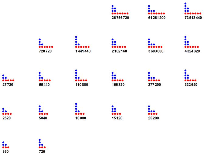
Figure 6 consists of multiplicity diagrams D(a(n)) for 1 ≤ n ≤ 13, showing the largest Chernoff divisor ч(ω(a(n))) in red, and the quotient k = a(n)/ч(ω(a(n))) in blue.
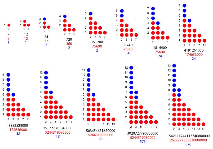
Click here to see a multiplicity diagram of a(120) = K(30) × ч(90) in the style of Figure 6. These numbers have 713, 107, and 607 decimal digits, respectively. This diagram has the advantage of more crisply defining the characteristic Idaho-like prime shape exhibited in a(n).
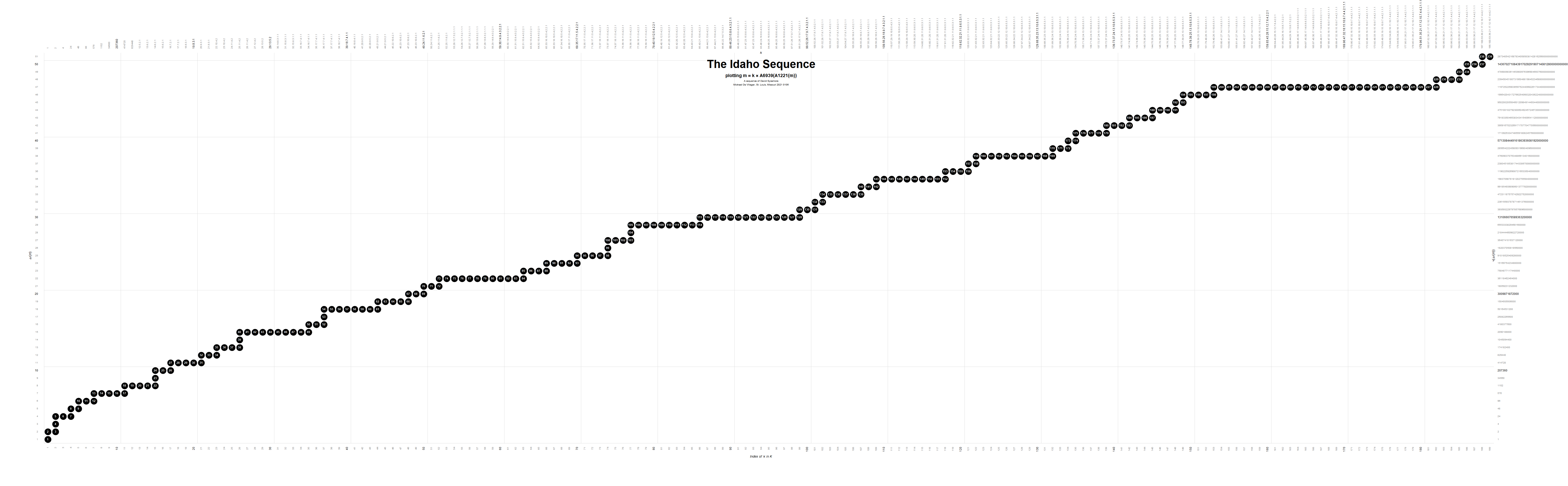
We may plot the terms m = K(x) × ч(y) at (x, y), The coordinates (x, y) can be used to succinctly specify a distinct term m in a(n).
We note that the terms of the sequence are produced in order by applying increment to either x or y as n increases. In other words, either the greatest Chernoff divisor index y advances (which is tantamount to ω(a(n))), or the primitive k factor index x advances. Therefore, given the Chernoff sequence A6939 and the primitive k factor sequence K, we can represent the sequence perhaps even more simply by reducing it to a characteristic function we already examined. The sequence d(n) = 1 when ω(a(n + 1)) = ω(a(n)) + 1. This is equivalent to the first differences of ω(a(n)), that is, the mappings of A1221(n) across a(n). Where we have “1”, we increment y, otherwise we increment x and thereby via K(x) × ч(y), ably reproduce the sequence a(n).
Figure 7 is a plot as described above. Click here for a poster-size enlargement that shows 240 terms.
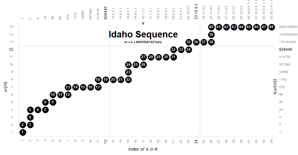
Figure 8 is a plot of L(n) = ω(a(n)) for 1 ≤ n ≤ 212, which is a simplified version of Figure 4 and its enlargement.
Divisibility of the Idaho numbers.
We observe the intersection of the Idaho numbers and the highly composite numbers include the first 5 terms. Therefore we may gather that the Idaho numbers are fairly divisible numbers.
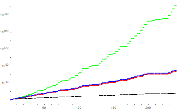
Figure 9 as a plot of the divisor counting functions of the largest HCN m < a(n) in green, the Idaho number a(n) in blue, the greatest Chernoff divisor ч(ℓ) | a(n) in red, and the greatest primorial divisor P(n) | a(n) in black for 0 ≤ n ≤ 240.
Binary compactification of m.
We understand that the terms m tend to be large. Indeed, a(146) has 1005 decimal digits. We might better understand the numbers m via their multiplicity notation M(m), noting indeed the length of this notation ℓ = ω(m), which indeed also proves lengthy.
The reduction of a(n) by the greatest Chernoff divisor ч(ω(a(n))) does not admit compactification in and of itself, since the quotient k is ambiguous as to the original term, though, given the values in K(x) and an algorithm that renders ч(y), we may store the coordinates (x, y) in the above plot and reconstruct the terms in this sequence.
We can compactify the terms, citing the 5th “basic fact” we listed above, i.e., that the multiplicities e are distinct. Therefore we may sum the mappings f(n) = 2(n − 1) across the e in M(m) and obtain the decimal value of a binary number that is much smaller than m.
For instance, we may compactify the number a(5) = 151200 as follows:
a(5) = 151200 = 25 × 33 × 52 × 71.
Multiplicities are
(5, 3, 2, 1) → 2(5 − 1) + 2(3 − 1) + 2(2 − 1) + 2(1 − 1) = 16 + 4 + 2 + 1 = 23.
We note that 23 = 101112, therefore we have recorded the multiplicities of the primes in the position of 1s in the binary notation of 23. We can recreate a(5) by writing these positions in descending order and then raising prime(i) to the multiplicity in the i-th place in the list.
Therefore we create the sequence b(n) = Sum_{j = 1..ℓ} 2(ej − 1) = Sum_{j = 1..A089576(n)} 2(A347285(n, j) − 1) = A347287(n):
0, 1, 3, 5, 11, 23, 39, 75, 151, 279, 559, 1071, 2127, 4255, 8351, 16687, 33327, 66095, 132191, 263263, 526511, 1052847, 2101423, 4202847, 8405695, 16794303, 33587903, 67175807, 134284671, 268568959, 537004415, 1074006399, 2148012799, 4295496447, 8590992639, 17181985279, ...
The compactification is sufficient to store 3322 terms in a standard OEIS b-file, whereas, through storing the decimal values of a(n) in the usual way we can only manage 145 terms. We can decode the b-file by taking r, the reverse of the union of positions of 1s in the binary notation of b(n), and mapping these as exponents for prime(i) where i is the position of the exponent in r.
Table 2 lists some of the basic parameters of the smallest terms of a(n). Column 1 contains m = a(n) = A347284(n). Column 2 lists k(n) = A347356(n) = a(n)/ч(n) = A347284(n)/A6939(n). The binary compactification b(n) = A347287(n) of exponents of prime power factors of a(n) appears in the third column. Index n is in the center, followed by ω(a(n)) = A1221(A347284(n)) = A089576(n). M(m) = A067255(A347284(n)) = row n of A347285. Finally, M(k) = A067255(A347356(n)).
m = a(n) k b(n) n ω(m) M(m) M(k)
---------------------------------------------------------------------------
1 1 0 0 1 0 0
2 1 1 1 1 1 0
12 1 3 2 2 2.1 0
24 2 5 3 2 3.1 1
720 2 11 4 3 4.2.1 1
151200 2 23 5 4 5.3.2.1 1
302400 4 39 6 4 6.3.2.1 2
1814400 24 75 7 4 7.4.2.1 3.1
4191264000 24 151 8 5 8.5.3.2.1 3.1
8382528000 48 279 9 5 9.5.3.2.1 4.1
251727315840000 48 559 10 6 10.6.4.3.2.1 4.1
503454631680000 96 1071 11 6 11.6.4.3.2.1 5.1
3020727790080000 576 2127 12 6 12.7.4.3.2.1 6.2
1542111744113740800000 576 4255 13 7 13.8.5.4.3.2.1 6.2
3084223488227481600000 1152 8351 14 7 14.8.5.4.3.2.1 7.2
92526704646824448000000 34560 16687 15 7 15.9.6.4.3.2.1 8.3.1
555160227880946688000000 207360 33327 16 7 16.10.6.4.3.2.1 9.4.1
...
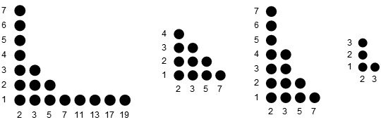
Figure 10 is a comparison of the prime shapes of A2182(80) = 27935107200 at left, A6939(4) = 75600, a(7) = 1814400, and a(7)/A6939(4) = 24 at right.
Other means of compactification.
Because the numbers m in a(n) become large quickly as n increases, we seek ways of storing terms in a succinct manner.
Tipping Idaho.
The first thought regards taking the conjugate of M, that is, the primorial factor notation of m and read it instead as multiplicity. This would transmute a(8) = 1814400 = 27 × 34 × 52 × 71 ⇒ 24 × 33 × 52 × 72 × 11 × 13 × 17 = 1286485200. This sequence c(n) begins:
1, 2, 12, 60, 2520, 831600, 10810800, 1286485200, 8066262204000, 185524030692000, 14687937509885640000, 455326062806454840000, 286400093505260094360000, 515374104261780487199876400000, 22161086483256560949594685200000, 311429748349204451024654111115600000
Generally, we have larger numbers in c(n). The move initially was designed to reduce the largest multiplicity, but additionally, we have duplicated multiplicities that stem from the tall Idaho mast (2n) become tail of 1s. Therefore we no longer enjoy the amenity of an unambiguous binary compactification.
Bitmap storage.
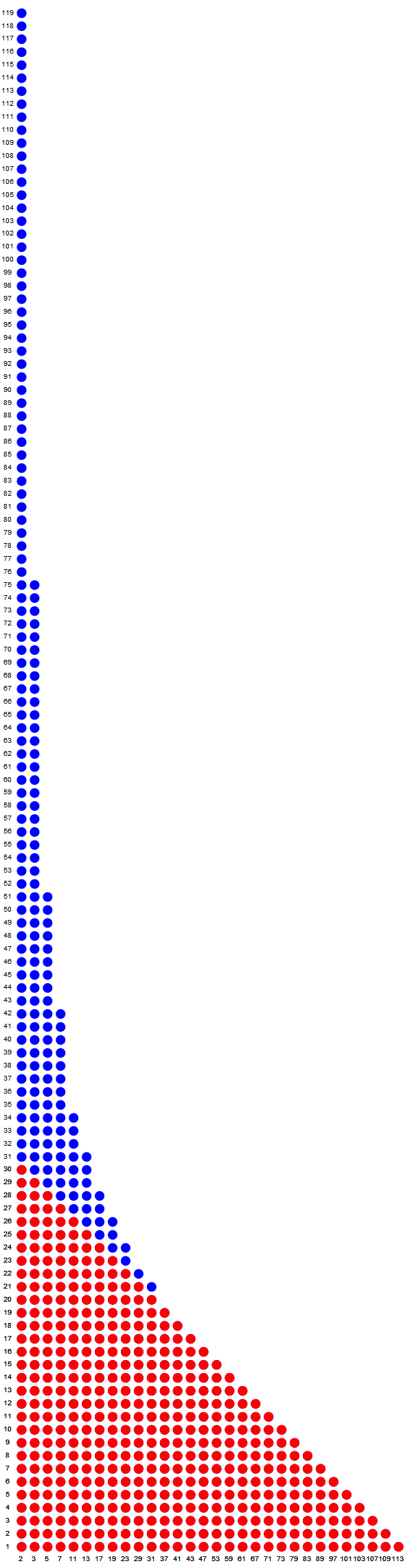
Now we consider stepping back from full binary compactification to instead plot the datum b(n) = A347287(n) read as binary digits in order of their exponents. Thus, a(8) = 1814400 = 27 × 34 × 52 × 71 ⇒ b(8) = 75 = “1001011”2, thus we plot the datum “1, 1, 0, 1, 0, 0, 1”, padded by zeros signifying “off” pixels as necessary to create a raster of b(n) across arbitrary 1…n. We know that the datum b(n) will have length n since the greatest multiplicity in a(n) = n. Hence we can set the target size of the raster and efficiently pad each datum to the final size during generation.
The resultant image can be used to store the binary numbers in raster form where each datum is an entry in b(n), which can then be processed to read the positions ej of 1s in a given datum n, in reverse order of magnitude, as exponents ej of prime( j), the prime powers thus multiplied to reproduce a(n). Thereby we store the sequence as a bitmap.
Figure 11 is a bitmap that displays b(n) with bits reversed, as a datum, for 1 ≤ n ≤ 512. Click here for an enlarged raster covering 1 ≤ n ≤ 4096, and here for an enlarged image covering 10000 terms.
The image is delightful in appearance and registers the trajectories of multiplicities of particular primes, the rightmost in the image pertaining to prime 2, its horizontal translation represents its multiplicity, followed leftward by 3, then 5, etc. We note the spacings of the trajectories generally telegraph the magnitude of prime spacings.
Emergence of negative space in the bitmap.
Our attention in such an image perhaps turns to the first emergence of prime gaps as single pixels. The emergent “negative space” that shows as white in the image between two areas of black indeed are occasions where the first differences increase from 1. Therefore we can identify n such that the gap between pi and p(i + 1) first emerges.
In essence, we are concerned with the least n for which the adjacent multiplicity difference
e(j + 1) − ej > 1.
Table 3 lists the first emergence of the prime gap between pj and p(j + 1). (Click here for an extended list using a dataset of the smallest 10000 Idaho numbers).
i p_j n
---------------
1 2 3
2 3 7
3 5 15
4 7 20
5 11 59
6 13 45
7 17 118
8 19 80
9 23 75
10 29 264
11 31 119
12 37 205
13 41 449
14 43 262
15 47 210
16 53 253
17 59 758
18 61 305
19 67 489
20 71 1004
21 73 384
22 79 617
23 83 462
24 89 400
25 97 817
26 101 1631
27 103 891
28 107 1796
29 109 974
30 113 357
31 127 1186
32 131 847
...
It is clear that these gaps broaden as n increases as a consequence of distinct primes.
Tracing the trajectory of multiplicities ej.
Likewise, we may extract functions f(j, n) = ej associated with the multiplicities of pj | a(n) that remain undefined (or by convention assigned the value 0) until that n which has a particular pj | n, i.e., while j > ℓ = ω(a(n)). The plot of these functions would correspond with an individual trajectory of the multiplicity ej of prime pj in Figure 7, and the height of the j-th column in a multiplicity diagram D(a(n)). Hence we can view a(n) through the lens of a particular prime pj, perhaps thus obtaining sequences a( j, n) = pjej, where j is the prime index. Thus, a(n) represents the product of all of these individuated prime power sequences.
By definition f(1, n) = n.
f(2, n) begins:
1, 1, 2, 3, 3, 4, 5, 5, 6, 6, 7, 8, 8, 9, 10, 10, 11, 11, 12, 13, 13, 14, 15, 15, 16, 17, 17, 18, 18, 19, 20, 20, 21, 22, 22, 23, 23, 24, 25, 25, 26, 27, 27, 28, 29, 29, 30, 30, 31, 32, 32, 33, 34, 34, 35, 35, 36, 37, 37, 38, 39, 39, 40, 41, 41, 42, 42, 43, 44, 44, 45, 46, 46, 47, ...
which have run lengths r(2, n):
2, 1, 2, 1, 2, 2, 1, 2, 1, 2, 2, 1, 2, 1, 2, 1, 2, 2, 1, 2, 1, 2, 2, 1, 2, 1, 2, 1, 2, 2, 1, 2, 1, 2, 2, 1, 2, 1, 2, 1, 2, 2, 1, 2, 1, 2, 2, 1, 2, 1, 2, 2, 1, 2, 1, 2, 1, 2, 2, 1, 2, 1, 2, 2, 1, 2, 1, 2, 1, 2, 2, 1, 2, 1, 2, 2, 1, 2, 1, 2, 1, 2, 2, 1, 2, 1, 2, 2, 1, 2, 1, 2, 1, 2, 2, ...
and the greatest term appears to be 2.
r(3, n) begins:
1, 3, 2, 3, 2, 3, 2, 3, 1, 3, 2, 3, 2, 1, 4, 1, 3, 2, 3, 2, 3, 1, 4, 1, 3, 2, 3, 2, 1, 3, 2, 3, 2, 3, 2, 3, 1, 3, 2, 3, 2, 1, 4, 1, 3, 2, 3, 2, 3, 1, 4, 1, 3, 2, 3, 2, 1, 3, 2, 3, 2, 3, 1, 4, 1, 3, 2, 3, 2, 3, 2, 1, 3, 2, 3, 2, 3, 1, 4, 1, 3, 2, 3, 2, 1, 3, 2, 3, 2, 3, 1, 4, ...
with greatest term 4.
The sequence of greatest terms of r(j, n) begins:
1, 2, 4, 5, 8, 10, 13, 16, ...
The tracing of individual f(j, n) admits an ability to plot the multiplicities of any prime pj as n increases, if desired.
Efficacy of bitmap compactification.
The primary point of the bitmap, however, is the succinct storage of a large number of terms in a picture, which is indeed achieved to excellence by the enlarged 4096-term image, which weighs 115 kb, yet bests the 1.6 Mb binary compactification of 3322 terms in a txt file. (The 10000-term image weighs 479 kb.)
Code 3 provides a way to extract terms of a(n) from the bitmap, while Code 4 offers a means to generate the bitmaps. The extraction of data from the file is efficient once the image is loaded; indeed we are able to reconstruct the very largest term in the enlarged image in a fraction of a second, i.e., a(4096), a number with 373370 decimal digits. Likewise, using the 10000-term image, we resuscitate a(10000), a number with 1937824 decimal digits nearly as quickly.
Hence, the storage of numbers m in a(n) is only bounded by the practicality of bitmap size. Given current parameters, using the largest possible raster size in Adobe Photoshop today, we can store up to 30000 terms in a bitmap, if we are able to generate them. An image of great size may introduce data processing delays and other issues, therefore at some point we have a practical limit toward the storage of the large numbers in this sequence. For this reason we have decided that a 10000 term dataset is about as large as we’ll produce.
Recall that this image methodology is tantamount to the storage of the binary-compactified terms b(n), but in the form of pixels. It is available whenever we can apply binary compactification.
The compactification of numbers m in this sequence in a bitmap offers advantages over and above that of standard decimal positional notation.
We write numbers in decimal positional notation for the ability of such to succinctly convey exact information regarding numbers we encounter every day. This notation is not always efficaceous, here, especially, when the numbers in question are large.
We should bear in mind that the Idaho numbers are special in that they admit such representation, as they are in A025487, the multiplicities ei of their prime divisors pi are distinct and strictly decrease as i increases. This compression methodology is not available to most integer sequences.
Given the definition of this sequence as a series of prime power factors, multiplicity notation is one method of specifying the numbers m, but even this method faces challenge given a great number of prime power factors. The binary compactification method reduces the size of the numbers at the expense of muddying human understanding of the nature of the prime power factors, while machines can indeed extract and reconstruct the numbers for analysis.
The expression of the distinct multiplicities ej = k by pixels at the k-th position takes advantage of the special nature of the numbers m in this sequence and admits ready access to each prime power factor, eliminating the need for obtaining the prime power decomposition of a large decimal number. Basic parameters — ω(m), the distinct magnitude of each multiplicities ej, can be retrieved and processed with little engagement of computationally expensive factorization angorithms.
Hence the storage of m in a bitmap grants us additional versatility that storage as a decimal or binary-compactified number written in decimal may afford.
Because of the special nature of m in this sequence, we are able to store a large number of terms in a versatile way using bitmaps.
Compactification based upon a(n) as a product of primorials.
We recall the sequence q(n) = A347354(n) which is a list of primorial indices such that:
a(n) = Product_{k=1..n} P(q(n)) = Product_{k=1..n} A2110(q(n)).
Indeed, the conjugate of reverse-sorting the terms q(n) for 1 ≤ k ≤ n reconstructs the multiplicities ej for 1 ≤ j ≤ ℓ, since q = a(n+1)/a(n) can be rewritten a(n+1) = q × a(n). Thus, q(n) serves as an unsorted list of indices of all primorials P(q(k)) for 1 ≤ k ≤ n that produce a(n). Or, rather, the ordering is such that the product resulting from the first n indices is a(n).
The fact that the iteration of ej may only occur if and only if e(j − 1) has incremented enables the generation of 212 terms in less than a minute using Code 5. We generated 214 terms of q(n) in 263 s, from which we can construct a(16384), a number with 4785473 decimal digits and ω(a(16384)) = 1646. Further, we generated 216 terms of q(n) in 7643 s, from which we can construct a(65536), a number with 64329225 decimal digits and ω(a(65536)) = 5587.
Table 4 lists the number of decimal digits and the number of distinct prime divisors of a(2k), and the number of decimal digits of τ(a(2k)).
k Len(m) ω(m) Len(τ(m))
-----------------------------------
1 2 2 2
2 3 3 2
3 10 5 3
4 24 7 6
5 82 12 10
6 245 19 20
7 725 30 39
8 2689 54 78
9 8758 91 155
10 29780 158 309
11 108788 286 617
12 373370 503 1234
13 1327007 905 2467
14 4785473 1646 4933
15 17401837 3015 9865
16 64329225 5587 19729
17 236946059 10356 39457
18 875414218 19267 78914
19 3258645311 36054 157827
20 12190758933 67753 315654
...
Table 5 lists the number of decimal digits, the number of distinct prime divisors of a(10k), and the number of decimal digits of τ(a(10k)).
k Len(m) ω(m) Len(τ(m))
----------------------------------
0 1 1 1
1 15 6 4
2 551 27 31
3 28578 155 302
4 1937824 1080 3011
5 141795119 8118 30104
6 11134582700 64877 301031
...
Thus, from q(n) we can construct a(k) for 1 ≤ k ≤ n; it is the most compact method of storing the numbers in this sequence. Having obtained 216 terms of q(n), we can store more data than is practical in a bitmap and for less storage space. Code 6 can be used to generate a(n) from q(n) stored at this site. Code 7 can be used to construct a single m in a(n).
The reconstruction of a(n) from q(1..n) yields a dataset that exceeds the ability of most computers to manipulate, however we manage to take samples of select tracts and numbers.
Looking at the number of decimal digits of τ(a(1000000)) = 301031, and that in reviewing the number of bits of τ(a(2k)) = 2k + 2, one might make a conjecture that the number of base-b digits in τ(a(bk)) = ⌈bk × logb 2⌉. We have not explored this aspect any further.
Variants of this sequence.
a(n) as a number triangle T(n, j).
The sequence a(n) is the product of all pjej < p(j − 1)e(j − 1), with p1e1 = 2n, for 1 ≤ j ≤ ℓ. Alternatively we might produce a triangle T(n, j) = row n of A347288 that lists pjej for 1 ≤ j ≤ ℓ:
Table 6 lists the first 24 rows of T(n, j):
n p_j^e_j
-------------------------------------
0 1;
(by definition)
1 2;
2 4, 3;
3 8, 3;
4 16, 9, 5;
5 32, 27, 25, 7;
6 64, 27, 25, 7;
7 128, 81, 25, 7;
8 256, 243, 125, 49, 11;
9 512, 243, 125, 49, 11;
10 1024, 729, 625, 343, 121, 13;
11 2048, 729, 625, 343, 121, 13;
12 4096, 2187, 625, 343, 121, 13;
13 8192, 6561, 3125, 2401, 1331, 169, 17;
14 16384, 6561, 3125, 2401, 1331, 169, 17;
15 32768, 19683, 15625, 2401, 1331, 169, 17;
16 65536, 59049, 15625, 2401, 1331, 169, 17;
17 131072, 59049, 15625, 2401, 1331, 169, 17;
18 262144, 177147, 78125, 16807, 14641, 2197, 289, 19;
19 524288, 177147, 78125, 16807, 14641, 2197, 289, 19;
20 1048576, 531441, 390625, 117649, 14641, 2197, 289, 19;
21 2097152, 1594323, 390625, 117649, 14641, 2197, 289, 19;
22 4194304, 1594323, 390625, 117649, 14641, 2197, 289, 19;
23 8388608, 4782969, 1953125, 823543, 161051, 28561, 4913, 361, 23;
24 16777216, 14348907, 9765625, 5764801, 1771561, 371293, 83521, 6859, 529, 29;
...
The triangle consists of numbers in A961 by definition. Each number in A961 appears at least once in the triangle. Additionally, many of the qualities studied regarding a(n) apply to T(n, j). The 145 terms of a(n) we can store decimally in the OEIS (i.e., including terms that have no more than 1000 decimal digits) equate to 2931 terms of the triangle, yet we can store 3321 rows of data or 769839 terms of the triangle that have up to and including 1000 decimal digits.
Sequence g(n) holding ej < 2n.
Initially, when presented with the notion of a(n), the author had improperly coded the sequence and instead, all prime divisors were not to exceed the first-established prime divisor 2n.
Let g(n) = p1e1 × p2e2 × … pℓeℓ where e1 = n and ℓ is the maximum possible number of consecutive prime divisors p subject to a condition on the exponents which requires that the exponent ej > 0 is the greatest possible integer for which pjej < p1n for all j ≤ ℓ. We observe that ℓ = π(2n) = A720(2n). This sequence begins:
1, 2, 12, 840, 720720, 144403552893600, 1182266884102822267511361600, 13353756090997411579403749204440236542538872688049072000, ...
Terms 0 ≤ n ≤ 6 are highly composite and superabundant; g(7) is superabundant.
Figure 12 consists of multiplicity diagrams of terms 2 ≤ n ≤ 7 of g(n).
This sequence lacks the connection with the Chernoff numbers, though we can certainly find a greatest Chernoff divisor of g(n). Binary compactification is not available since we see repeated multiplicities of prime divisors p | g(n). The numbers become large faster than those in a(n) as n increases. The multiplicity diagrams show that m in g(n) exhibit a long “tail” of large prime divisors p¹.
Conclusion.
The sequence a(n) is of interest on account of some of the curious properties of the prime power decomposition of its terms.
The sum S of the first differences of the multiplicities of the prime divisors of a(n) is (1 − n).
8. Let T be the sum of the first differences of the prime powers pe arranged in order of p. The sum 2n + T = 1 for n > 2.
Regarding the curious manifestation of the “Idaho” prime shape, we note that the multiplicity diagram features a skew that features a precipitous fall from 2n across p > 2 where it tapers into the greatest Chernoff divisor’s prime shape since for 1 ≤ j ≤ ℓ, the multiplicity ej ≥ ℓ − j + 1. Additionally, the terms m in a(n) are products of primorials. We can obtain a pair of coordinates (x, y) so as to identify a distinct term m in a(n) via K(x) × ч(y), and using L(n), the first differences of the ω(n) function mapped across the terms of a(n). Furthermore, since the multiplicities e are distinct, we can compactify the multiplicities e of the primes p | a(n) using the number b(n) = Sum_{j = 1..ℓ} 2(ej − 1). Furthermore, we may efficiently store the binary compactification data in a large bitmap that has its own interesting properties. The storage of the multiplicities ej in the prime power factors pjej | m grants us versatility in studying the relationships between the distinct multiplicities.
Afterword.
Naohiro Nomoto (Chiba, Japan) posed A089576 on 29 December 2003. Richard J. Mathar wrote on 8 September 2021, upon encountering erstwhile A347286 (which was understandably recycled as a duplicate of Nomoto’s long-extant sequence):
“The steps are a downward recursion in the prime powers: start at 2n in A961, i.e., at A961(A024622(n)); skip to the left to the next smaller power 3e_3 (see A024623), then to the left to the next smaller power 5e_5, to the left to the next smaller power 7e_7 etc., and count the steps to reach 1.”
Hence, though David Sycamore arrived at the notion of A347284 independently, thoroughly analyzed by the author, Naohiro Nomoto must have considered the “Idaho” notion 17 years before. Indeed, the notion R. J. Mathar had described would seem to have been considered perhaps many times before by many people. The writing of A347286 uncovered the fact that Nomoto had been here first. Hence, we acknowledge Naohiro Nomoto’s pre-existing contribution to the concept of the “Idaho” numbers.
Finally, we thank Dr. Mathar for his input regarding A089576 and what he had written in that sequence’s commentary.
Appendix:
Code 1: Generate a(n) = A347284(n):
Array[Times @@
NestWhile[
Append[#1, #2^Floor@ Log[#2, #1[[-1]]]] & @@ {#,
Prime[Length@ # + 1]} &, {2^#}, Last[#] > 1 &] &, 2^12, 0]
Code 2: Generate the Chernoff numbers ч(n) = A6939(n):
Array[Product[Prime[i]^(# - i + 1), {i, #}] &, 12, 0]
Code 3: Generate the first terms of a(n) for 1 ≤ n ≤ 120 from the image in Figure 11*:
With[{r = ImageData@ Import["http://www.vincico.com/seq/s20210106-7.png"]},
Array[Times @@ Flatten@ MapIndexed[Prime[#2]^#1 &, #] &@
Reverse@ Position[r[[#]], 0.][[All, 1]] &, 120]]
*This code can be altered to pull all a(n) for 1 ≤ n ≤ 4096 from the enlarged image by changing the target url file to “s20210106-7a.png”, or use “s20210106-9.png” to take advantage of a 10000 term dataset. We have pulled the largest term from the enlarged image over the internet and it takes a fraction of a second (given a good connection) to regenerate the term. Reconstructing a(n) for 1 ≤ n ≤ 4096 from the enlarged image takes about a minute.
Code 4: Create your own bitmap of a(n) for 1 ≤ n ≤ 1024 in the style of Figure 11*:
Monitor[Block[{a = {}, b, i, m, p, q, nn = 2^10, r},
r = ConstantArray[0, nn];
Do[b = {k};
Do[If[Last[b] == 1, Break[], i = 1;
p = Prime[j - 1]; q = Prime[j];
While[q^i < p^b[[j - 1]], i++];
AppendTo[b, (i - 1)]], {j, 2, k}];
AppendTo[a, ReplacePart[r, Map[# -> 1 &, b]]], {k, nn}];
ColorNegate@ Image@ a], k]
*Please note that generating a large bitmap may require a lot of time! The 4096 × 4096 image required about 2 hours to produce. Your computer configuration and performance may impact success in generating these images.
Code 5: Fast code to generate a(n):
Block[{nn = 2^12, a = {}, b, e, i, m, p},
Array[Set[e[#], 0] &,
Floor[2^# If[# <= 4, 1/2, -1 + 2^(7/(3 #))]] &[Ceiling@ Log2@ nn] ];
Do[e[1]++; b = {2^e[1]};
Do[If[Last[b] == 1, Break[], i = e[j]; p = Prime[j];
While[p^i < b[[j - 1]], i++];
AppendTo[b, p^(i - 1)]; If[i > e[j], e[j]++]], {j, 2, k}];
AppendTo[a, Times @@ b], {k, nn}];
Prepend[a, 1]
]
This index-memoized approach produces 212 terms in 30.6563 s, whereas Code 1 produces same in 37.4844 s. A version that stops incrementing subsequent multiplicities when ej hasn’t changed is just slightly less efficient at 30.6719 s.
Code 6: Generate a(n) for 0 ≤ n ≤ 120 from q(n) = A347354(n) stored on this site*:
Block[{s = Import["http://www.vincico.com/seq/s20210106q.txt", "Data"][[All, -1]]},
{1}~Join~Array[Times @@ Flatten@ MapIndexed[Prime[#2]^#1 &,
Table[LengthWhile[#1, # >= j &], {j, #2}] & @@ {#, Max[#]} ] &@
ReverseSort@ s[[1 ;; #]] &, 120]]
*One should take care not to flood memory with large numbers; we haven’t maintained the 65536 term dataset in RAM, but instead selected certain numbers based on properties when studying this sequence. A 10000 term dataset has been kept in RAM.
Code 7: Generate a(12) from q(n) stored on this site*:
Block[{n = 12, s = Import["http://www.vincico.com/seq/s20210106q.txt", "Data"][[All, -1]]},
Times @@ Flatten@ MapIndexed[Prime[#2]^#1 &,
Table[LengthWhile[#1, # >= j &], {j, #2}] & @@ {#, Max[#]} ] &@
ReverseSort@ s[[1 ;; n]] ]
*One should take care not to flood memory with large numbers; a(65536) has 64329225 decimal digits! It may be better to obtain an aspect of large decimal numbers rather than construct the decimal number itself. Normally these are much smaller numbers, however, the number of divisors of a(65536), for example, still has 18565 decimal digits, and we calculate such via the exponents of the prime power factors that are already available via the conjugate of the reverse-sorted primorial factor indices stored in q(n), rather than by taking DivisorSigma[0, #] of the reconstructed multimillion decimal digit number, which would require a lot of time. It is our experience that the examination of very large terms of this sequence, beyond aggregate qualities, is unnecessary.
Concerns OEIS sequences:
A000079: Perfect powers of 2 (the largest prime power divisors of a(n))
A000720: π(n) = Number of primes p ≤ n.
A000961: 1 and the prime powers pk with k ≥ 1.
A001221: ω(n) = Number of distinct prime divisors of n.
A002110: The primorials.
A002182: Highly composite numbers (HCNs), i.e., where records are set in A5.
A004394:
Superabundant numbers: n such that σ(n)/n > σ(m)/m for all m < n.
A006939:
Chernoff numbers ч(n).
A025487: List giving least integer of each prime signature; also products of primorial numbers.
A055932: Numbers where all prime divisors are consecutive primes starting at 2.
A067255: Multiplicities of prime divisors pk | n written in the k-th position, where k is the prime index.
A089576: ω(a(n)) = ℓn. Row lengths of A347285.
A347284: The “Idaho” numbers a(n).
A347285: Multiplicities of distinct prime divisors p | a(n): rows have n followed by ek = ⌊(log_pk(p(k−1)e(k−1))⌋ such that ek > 0.
A347287: b(n): Binary compactification of a(n): Sum_{k=1..ℓ} of 2(T(n,k)−1).
A347288: Prime power factors pe | a(n): rows have 2n followed by pkek with ek = ⌊(log_pk(p(k−1)e(k−1))⌋ such that ek > 0.
A347354: q(n): Primorial-index compactification of a(n). Sum of T(n,k) − T(n-1,k) for row n of A347285.
A347355: Indices k of records in A347354, or occasions k such that A089576(k) = A347354(k).
A347356: K(n) = a(n)/ч(ω(a(n))) = A347284(n)/A6939(A089576(n)).
Document Revision Record.
2021 0106 2200
Draft 1.
2021 0107 1530 Draft 2.
2021 0113 1730 Final draft.
2021 0408 1945 Typographical edit.
2021 0916 1230 OEIS edit, afterword.
2021 1013 1445 OEIS edits complete.