OEIS A336893
A sequence by David Sycamore, this page written by Michael Thomas De Vlieger, St. Louis, Missouri, 2020 0807.
Extension revision 2020 1111.
Introduction.
We define a(n) = A336893(n) as follows. Set a(1) = 1. Thereafter, for all n > 1, a(n) is the lexically earliest sequence with distinct nonzero positive integers k (not already in a(n)) such that the sum of decimal digits of the first n terms is coprime to their concatenation.
Therefore, for a(2), we consider k = 2, however, concatenating {1,2} yields 12, but 1 + 2 = 3 | 12, thus, we consider k = 3. We observe that 13 and 4 are coprime, thus a(2) = 3. For a(3), we consider k = 2. We observe that 6 | 132, and k = 3 is already in the sequence; k = 4 yields 8 and 134 with gcd(8, 134) = 2; k = 5 has 9 | 135, k = 6 has gcd(10, 136) = 2. For k = 7, we see that 11 and 137 are coprime, thus a(3) = 7, etc.
We denote “⊔” the concatenation operator, and “⍭” the sum-of-digits operator. Therefore, “c ⊔ k” denotes 10ℓc + k, where ℓ = ⌊1 + log10 k⌋ while “s ⍭ k” denotes the sum of s and the decimal digital sum of k. The numbers c and s arise recursively and contain the result of the last iteration of their respective functions. We exploit these facts so as to write an efficient algorithm to generate many terms of a(n).
The sequence a(n) begins (See Code 1.1):
1, 3, 7, 2, 4, 5, 9, 6, 13, 8, 19, 11, 15, 21, 10, 17, 22, 23, 12, 24, 25, 14, 27, 16, 20, 28, 26, ...
This link lists n, a(n) for 1≤ n ≤ 10000.
Since a(n) deals with digits, we consider the binary version of a(n), which we shall call b(n). This sequence begins (See Code 1.2):
1, 3, 5, 6, 7, 2, 9, 10, 11, 4, 13, 8, 12, 15, 17, 18, 20, 19, 14, 21, 22, 23, 24, 25, 16, 27, 30, ...
The focus of this paper is the decimal a(n), looking to the binary b(n) and versions of a(n) in alternate bases to attempt to explain some observed behavior of the decimal a(n).
Figure 1.1 is a plot a(n) for 1 ≤ n ≤ 1024 seen below in Figure 1.1 (see an enlarged plot of 3000 terms):
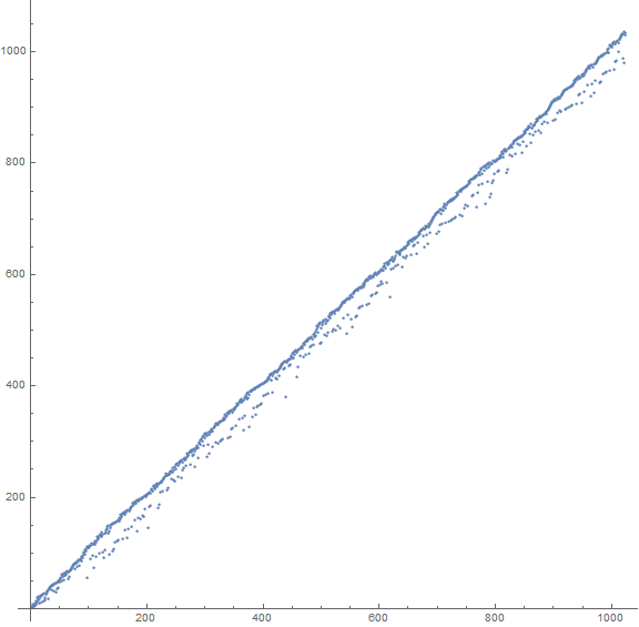
Here we note that the terms seem to generally follow the line n = a(n), with about a quarter of the terms falling more sparesly and significantly below this line. We note a sort of quasiperiodic “scalloping” between certain local lows in the fringe under the line with a “grain size” of about 200 at this scale.
Figure 1.2: We might compare this to the plot b(n) for 1 ≤ n ≤ 210 seen below in Figure 1.2 (see an enlarged plot of 212 terms):
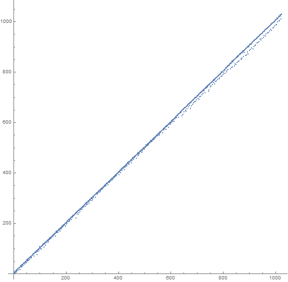
This graph resembles that of a(n).
Congruence Effects on Concatenation and Digit Sums.
Let us consider concatenation m ⊔ k, an operation on the digits of 2 numbers m and k expressed in base-b instead as a certain function C(m, k, b) = m × bℓ + k, where ℓ = ⌊1 + logb k⌋, i.e., the number of base-b digits necessary to represent k. Regarded algebraically, we see that the concatenation function thus can render the base b number c = m⊔ k as c ≡ k (mod bℓ). Since bℓ is a perfect power of b, we observe that numbers k coprime to bℓ are also coprime to b. Therefore we may regard the congruence c ≡ r mod b instead of c itself in certain operations.
We note that there are b(ℓ − 1) × φ(b) numbers k with ℓ base-b digits that are coprime to b, however, we may not apply k that are padded with leading zeros so as to maintain integer length ℓ; we may only append those k that have ℓ base-b digits that start with a nonzero digit, since k must appear in the sequence as an immutable base-b entry that does not feature leading zeros. Thus we are left with b(ℓ − 1) × φ(b) − ⌊b(ℓ − 2) × φ(b)⌋ numbers k that avoid leading zeros. For b = 10, we have 4, 36, 360, 3600, … valid terms k with 1, …, 4, … decimal digits that begin with a nonzero digit.
Let the function S(c, b) denote the sum of the base-b digits of k (expressed in base b). Likewise, we know that the decimal digit sum of c ≡ r (mod 9). Relatedly, we might regard S(c, b) ≡R (mod (b − 1) × be) for some integer e ≥ 0, reading 0 for c > 0 instead as (b − 1) × be.
Can we find a congruence relation that might simplify the sequence a(n) or b(n) and explain behavior? Since we are looking for gcd(C(m, k, b), S(c, b)) = 1, we might surmise that, unless we are identifying S(c, b) and C(m, k, b) belonging to different reduced residues of some immense primorial, we might not follow thought along these lines for the sheer complexity of such determination. We do observe the effects of reduced residues of primorials in a(n), which we will examine.
The Difference d(n) = a(n) − n.
The near-correspondence to n = a(n) and n = b(n) leads us to consider derivative sequences d(n) = a(n) − n and d2(n) = b(n) − n. These begin as noted:
d(n) = 0, 1, 4, -2, -1, -1, 2, -2, 4, -2, 8, -1, 2, 7, -5, 1, 5, 5, -7, 4, 4, -8, 4, -8, -5, 2, -1, 3, 0, ...
d_2(n) = 0, 1, 2, 2, 2, -4, 2, 2, 2, -6, 2, -4, -1, 1, 2, 2, 3, 1, -5, 1, 1, 1, 1, 1, -9, 1, 3, 1, 2, -4, ...
Figure 2.1 The plot of these sequences accentuate a cyclical pattern among numbers plotted above and below n = a(n) (or n = b(n)). Figure 3 shows d(n) (This link shows 10000 terms):
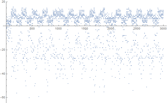
Figure 2.1 accentuates the “chatter” or “scalloping” seen in Figure 1.1, which we will term “crenellation” and examine in a later section.
Figure 2.2 shows d2(n) = b(n) − n for 1 ≤ n ≤ 212, akin to decimal a(n) − n of Figure 2.1:
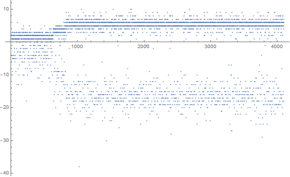
Notable here is the curious shift of the average value of terms greater than 0 between n approximately 637 and 836. This is reflected in the terms less than 0 in the plot.
Analysis of a(n).
We can find records r(n) in a(n) (and surely b(n)) as well as least unused numbers u(n) that are missing from a(n) while larger k appear in a(n). (See Codes 3.1-3.7 inclusive)
Figure 3.1 is a plot of a(n) for 1 ≤ n ≤ 100, showing the records in dark red and the least unused u(n) in dark blue. Further, we label the index n for a(n) = n, plotting these large and in black. We label the indices of numbers that set records for a(n) − n (plotted large in red), and n − a(n) (plotted large in blue). The recordsetters in a(n) − n we term “superior recordsetters” or more simply, superiors, and those of n − a(n) “inferior recordsetters”, hence, inferiors. Other data here is shown in a golden tone.
Figure 3.2 is a plot of a(n) for 1 ≤ n ≤ 1000, using the same color scheme and labeling, though not all the labels show as they are placed per algorithm. (See Code 3.6)
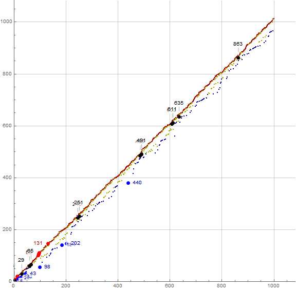
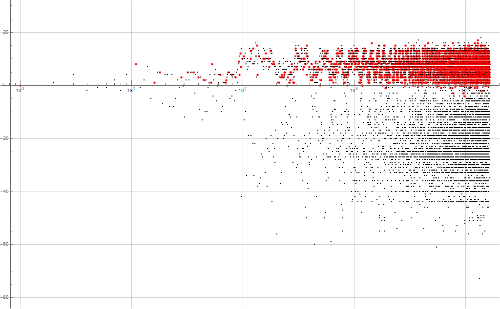
Figure 3.3 is a log plot of a(n) − n for 1 ≤ n ≤ 214, showing and labeling the superior and inferior recordsetters. See an enlarged log plot for 1 ≤ n ≤ 216. (See Code 3.7)
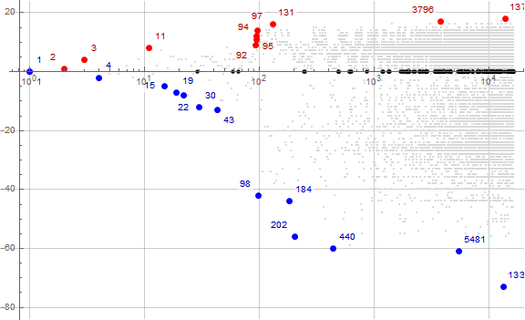
Figure 3.3 seems to suggest that a(n) remains rather tight around a line of slope 1 struck from origin across n in the smallest 4 orders of decimal magnitude. Within this domain, we always find u(n) within 100 units of a(n) − n.
Parity of a(n).
Let ℓ be the rank of the index n, i.e., ⌊1 + log10 n⌋, and let the “rank domain” be the interval 10e…(10(e + 1) − 1).
We observe in Figure 3.3 a dichotomy between “early” terms (a(n) > n) versus “tardy” terms (a(n) < n).
The indices n such that a(n) > n:
2, 3, 7, 9, 11, 13, 14, 16, 17, 18, 20, 21, 23, 26, 28, 31, 32, 33, 34, 35, 36, 38, 39, 40, ...
The indices n such that a(n) = n:
1, 29, 59, 65, 245, 251, 485, 488, 491, 608, 611, 635, 863, 1171, 1189, 1325, 1331, 1355, 1705, 1771, 1789, 1858, 1925, 1928, ...
The indices n such that a(n) < n:
4, 5, 6, 8, 10, 12, 15, 19, 22, 24, 25, 27, 30, 37, 41, 43, 46, 48, 49, 54, 58, 64, 66, 77, ...
Though the early terms hew closer to a(n) = n than the tardy, meaning that at least the outliers of the early subset tend to appear closer to than those of the late. However, if we divide the terms of a(n) according to their rank domain, we see that the number of early terms is around two-thirds, with few terms a(n) = n, and about 2/9 of the terms tardy.
rank domain early on-time tardy
----------------------------------
1..9 4 1 4
10..99 63 3 24
100..999 666 9 225
1000..9999 6618 100 2282
As to parity, there is a strong but incomplete dichotomy regarding the “earliness” of k (i.e., a(n) – n > 0), k “on schedule” (i.e., a(n) – n = 0), or the “tardiness” of k (i.e., a(n) – n < 0):
early on time tardy
rank domain even | odd even | odd even | odd
-------------------------------------------------
1..9 0 4 0 1 3 1
10..99 18 45 0 3 22 2
100..999 225 441 2 7 224 1
1000..9999 2217 4401 24 76 2258 24
There seems to be a statistical stability among the decimal ranks. Generally, about 2/9 evens and 4/9 odds early, 2/9 evens and 2/900 odds late, with 2/900 evens and 7/900 odds “on time”.
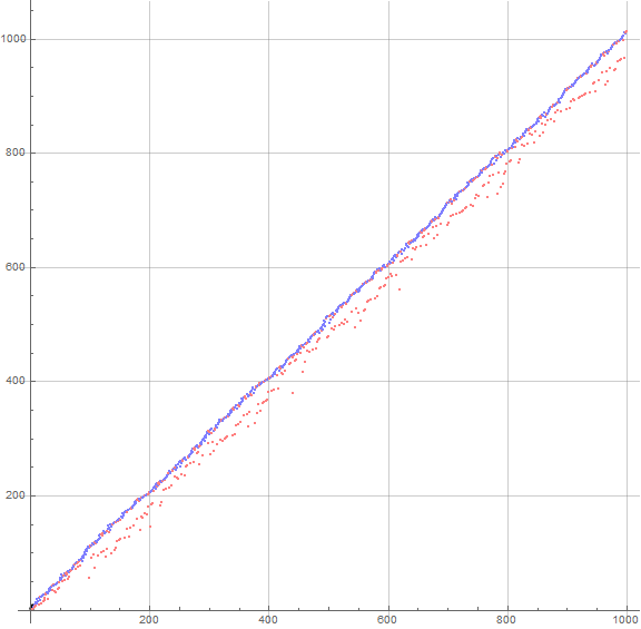
Figure 4.1 replots Figure 1.1, color-coding odd a(n) blue and even a(n) red, with 1 ≤ n ≤ 103. (Click here for a replot of Figure 2.3 showing parity in the same way for 1 ≤ n ≤ 216.)
Examining congruence mod 10, we derive the following regarding rank ranges.
residue 1 2 3 4
(mod 10) + . - + . - + . - + . -
----------------------------------------------------------
0 . . . 4 . 4 46 . 45 445 . 454
1 . 1 . 10 . 1 87 3 . 865 31 4
2 . . 1 4 . 4 45 . 45 449 2 449
3 2 . . 9 . . 88 1 1 883 13 4
4 . . 1 4 . 3 45 . 46 452 1 447
5 . . 1 8 1 1 87 3 . 862 26 12
6 . . 1 3 . 5 46 . 44 444 1 455
7 1 . . 10 . . 89 . . 898 1 2
8 . . . 3 . 6 43 2 44 427 20 453
9 1 . . 8 2 . 90 . . 893 5 2
For index rank domain 1, we have no terms that belong to 0 or 8 (mod 10). The earlies belong to 3, 7, and 9 (mod 10) and the lates consist of numbers belonging to 2, 4, 5, and 6 (mod 10). A number (1) is “on time” in this range and belongs to 1 (mod 10).
For index rank domain 2, we have coverage. Every residue (mod 10) appears early, with the odds about twice as common as evens. The residues 1 and 7 appear a bit more often, and the residues 6 and 8 appear a bit less often than an even distribution according to parity as described. For “on time” terms, we have one term belonging to 5 (mod 10), and 2 belonging to 9 (mod 10). For late terms, we have all residues represented except 7 and 9 (mod 10). The chart summarizes the findings.
We might examine rank ranges, rather than the index rank domains:
residue 1 2 3 4
(mod 10) + . - + . - + . - + . -
----------------------------------------------------------
0 . . . 6 . 3 79 . 11 769 . 131
1 . 1 . 8 . 1 66 3 21 695 31 174
2 1 . . 7 . 2 69 . 21 653 2 245
3 1 . . 8 . 1 68 1 21 710 13 177
4 . . 1 5 . 4 59 . 31 559 1 340
5 . . 1 6 1 2 75 3 12 737 26 137
6 . . 1 7 . 2 61 . 29 612 1 287
7 1 . . 5 . 4 74 . 16 737 1 162
8 . . 1 6 . 3 65 2 23 665 20 215
9 1 . . 5 2 2 50 . 40 481 5 414
This is an alternate, k-centered approach to “earliness” and “tardiness” versus a(n) – n positive, parity, or negative as in the last study. We examine numbers k in the rank range desired, and then assess where these fall, early or late, regardless of the rank domain. This shows that (generally) numbers that belong to 0, 3, 5, 7 (mod 10) appear early, and numbers belonging to 4 or 9 (mod 10) have a greater tendency to appear late.
The parity plot of a(n) – n clearly demonstrates an impure dominance of odd terms in the early region (i.e., a(n) – n > 0) and a more solidly even late region (i.e., a(n) – n < 0), especially the more tardy the term.
Let primorial P(n) = A2110(n), the product of the smallest n primes p.
If we are seeing odd a(n) early, might we instead be seeing a(n) that are generally belonging to a reduced residue of a primorial? This is a worthy consideration, since the reduced residues r of a primorial (i.e., r such that gcd(r, P(n)) = 1) harbor all primes q coprime to P(n).
In a plot of a(n) − n, the pattern of a(n) mod 3 looks mixed, but for a(n) mod 6, indeed we see a pattern, not particularly according to a(n) ≡ 0 (mod 6) (which appear strongly negative, thus tardy, on the plot of a(n) – n), but instead to a(n) ≡ ±1 (mod 6), which seem to appear nearly reliably early.
What seems to be happening as we build a(n) via (c ⊔ k) ⊥ (s ⍭ k) is that early k are more likely to be congruent to a residue r in the reduced residue system of a number that minimizes such residues, i.e., a primorial, so as to maximize the chance k ⊥ (s ⍭ k).
Therefore we see not only a stark parity preference for the “early” upper half of the plot of a(n) – n, but a preference for k ≡ r (mod P(i)) such that r ⊥P(n). This frames with the logical definition of the sequence.
Figure 4.2 is a plot of a(n) − n for n ≤ 100 examining congruence of k with a reduced residue of in the system of the largest primorial P(n) in the list {2, 6, 30, 210} (i.e., such that k mod P(n) is coprime to P(n)). Blue = 2, green = 6, orange = 30, and red = 210 (or larger). The terms in black have gcd(k, P(n)) > 1, which contains all the evens.
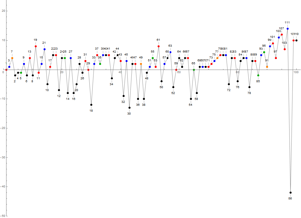
Figure 4.3 is a log plot of a(n) − n for 1 ≤ n ≤ 214 showing k in the RRS of the largest primorial that meets or exceeds the local record in a(n). We see that these appear generally above the x-axis.
The Proof of the Existence of the Sequence a(n).
Neil Sloane had asked whether the sequence a(n) always exists, given that, despite the closeness of these plots to a slope of 1 and all the data, no one seems to have proved that a grand concatenation coprime to the grand digit sum will always be found.
Sycamore attempted to answer this by trying to find an upper bound for k. De Vlieger’s search for a congruence-related method via the RRS of primorials was seen as cumbersome. We know that prime q > s is certainly coprime to s, since q cannot divide s that it exceeds, and that generally, primes must either divide or be coprime to another number. Sycamore observed that c is larger than s for n > 1, thus, he surmised creating a “backstop” prime q such that we are guaranteed to find k for all n. The algorithm v(n) for q is akin to that of A083754, except that, instead of being self-referential, v(n) would instead need to apply to a(n), thus, we have the potential to see the same q for different n, if q never appears in a(n).
OEIS A083754 begins with 1 and thereafter is the least novel k in A045572 (i.e., k ≡ ±1 or ±3 (mod 10)) such that appending k to the grand concatenation of preceding terms in A083754 results in a prime number. (See Code 5.1) It begins:
1, 3, 7, 11, 9, 27, 63, 31, 53, 21, 13, 83, 33, 39, 49, 51, 77, 87, 307, 29, 229, 281, 151, 173, 481, 41, 99, 157, 177, 17, 357, 213, 231, ...
For the purposes of a(n), we must instead consider novelty of k regarding a(n), and the grand concatenation of all previous terms in a(n). (See Code 5.2) Thus, the backstop sequence v(n) begins (see 800 terms of v(n)):
1, 3, 7, 11, 9, 11, 31, 19, 67, 29, 31, 17, 21, 33, 63, 77, 169, 153, 141, 121, 63, 117, 33, 123, 59, 93, 41, 193, 359, 223, 39, 267, 209, 61, 289, 51, 357, 329, 447, 111, ...
We can increment j to generate k in A045572 using the formula:
(5j + (3j + 2 mod 4) − 4)/2
Figure 5.1 plots v(n) in a color code to indicate k ≡r (mod 10). Magenta indicates k ≡ 1 (mod 10), orange Magenta indicates k ≡ 3 (mod 10), green k ≡ 7 (mod 10), and blue k ≡ 9 (mod 10). For reference, we show a(n) in gray at the very bottom of the plot.
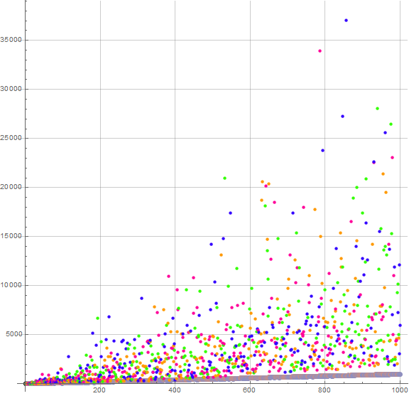
We see that there are only 2 primes in c(n), the sequence of concatenations of a(1)..a(n) for n ≤ 216; these are {13, 137}. The sequence v(n) − a(n) begins:
-, 0, 0, 9, 5, 6, 22, 13, 54, 21, 12, 6, 6, 12, 53, 60, 147, 130, 129, 97, 38, 103, 6, 107, 39, 65, 15, 162, 330, 205, 6, 230, 174, 22, 249, 10, 323, 287, 403, 68, ...
There are close approaches outside of 2 ≤ n ≤ 3, yet it seems that as n increases, there is a lower bound for v(n) that could be related to the spacing of large primes, since the grand concatenation c(n), if we are seeking the prime q, will be quite large.
However, we are not simply taking nextprime(c), but indeed, a sort of telescoping 10ℓc + k, where k has decimal digits and cannot admit leading zeros. Suppose we were able to somehow never generate a prime by incrementing j to produce sequential k ≡ ±1 or ±3 (mod 10), with 10ℓc of course increasing by a factor of 10 according to the decimal integer length ℓ? This question, however, does not constitute a proof, and the question remains, now, whether or not the backstop sequence exists.
A group of mathematicians that includes Maximilian Hasler, Max Alekseyev, and Charles Greathouse V had taken note of a(n) and suggested the proof does relate to the expected prime gap, involving A068695. From correspondence between Hasler and Sycamore, we have:
To find k such that N ⊔ k (concatenation) is prime, do the following:
let N' = 10N + 1 (this will guarantee that k starts with a leading 1 and not with leading 0’s which was missing in Max Al[ekseyev’]s proof).
Let t = ⌈(N' × 10r )1/3⌉ with r sufficiently large to guarantee that:
(1): (t + 1)³ starts with the digits of N (and not N + 1), then t³ will also start with the digits of N, even with the digits of N'.
(2): t is large enough so that there exists a prime between t³ and (t + 1)³
(look for Ingham in https://en.wikipedia.org/wiki/Prime_gap; it has been proved by Dudek that t > exp(exp(34)) is enough, see also A060199.)
Then any such prime will be of the form N ⊔ k where k starts with a nonzero digit ≥ 1.
A proof that either v(n) or a(n) always exists is beyond the scope of this work, though this team may furnish a proof in the coming days, posting it at A336893 and related sequences.
Crenellation in the plot a(n) − n.
We note the “crenellation” among both terms “above” and “below” the x axis in a scalar plot of a(n) − n which represents n = a(n). (See Code 1.3) The chatter above the axis seems to be confined to segments of n that are 100 wide, at first lower for odd ⌊ n/100 ⌋, then for 1000 < n < 2000, even ⌊ n/100 ⌋, etc. The “bookmatching” of the even-odd crenellations once n exceeds 1000 endures through n = 10000, i.e., we do not see bookmatching at that rank. It is not known whether we see bookmatching at n = 100000.
Figure 6.1 takes the mean of a(jn) for 1 < n < 1999 and 0 < j < 4, solely to amplify the pattern. We show a(jn) for n in the odd hundreds in blue, and even hundreds red.
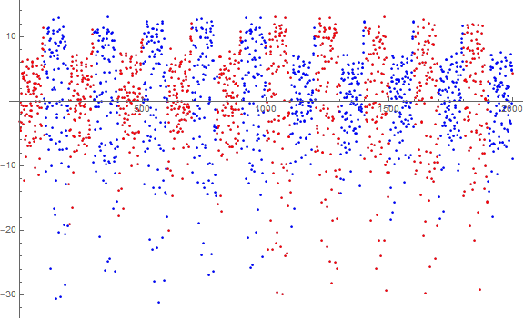
Note that the amplitude above the x-axis is reflected in a greater amplitude below the axis.
The sequence g(n).
Let s(n) be the grand digit sum of a(n), that is, the sum of all the decimal digits of a(1)..a(n). These are the grand digit sums s ⍭ k against which we attempt to find a coprime concatenation c ⊔ k. The sequence s(n) begins:
1, 4, 11, 13, 17, 22, 31, 37, 41, 49, 59, 61, 67, 70, 71, 79, 83, 88, 91, 97, 104, 109, 118, 125, ...
whereas c(n) begins:
1, 13, 137, 1372, 13724, 137245, 1372459, 13724596, 1372459613, 13724596138, 1372459613819, ...
Earlier we had observed that c(n) is greater than s(n) for n > 1 and we know c(n) ⊥ s(n) by definition of a(n).
We consider the sequence g(n) = gcd(a(n), s(n)), which is tantamount to gcd(k, s ⍭ k). The motivation for such consideration relates to attempting to find some pattern of congruence between k and s ⍭ k. This sequence begins (See Code 7.1):
1, 1, 1, 1, 1, 1, 1, 1, 1, 1, 1, 1, 1, 7, 1, 1, 1, 1, 1, 1, 1, 1, 1, 1, 1, 1, 1, 1, 1, 1, 1, 37, 1, 1, 1, 1, 17, 1, 1, 1, 1, 1, 1, 1, 1, 1, 1, 1, 1, 1, 11, 1, 1, 1, 1, 1, 1, 1, 1, 1, 1, 1, 1, 1, 1, 1, 1, 1, 1, 1, 1, 1, 1, 1, 1, 1, 1, 1, 1, 1, 1, 1, 1, 1, 1, 1, 1, 1, 1, 1, 1, 1, 1, 1, 1, 1, 1, 7, 1, 1, 1, 1, 1, 1, 1, 1, 1, 37, 1, 1, 1, 1, 1, 1, 43, 1, 1, 1, 1, 1, ...
Figure 7.1 plots g(n) for 1 < n < 300, highlighting g(n) > 1 in red and annotating many of the instances.
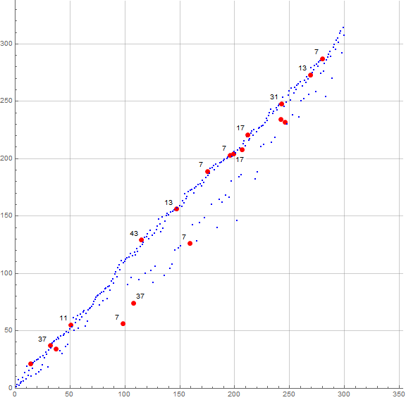
Though it appears from the data shown that g(n) is either 1 or prime, we find prime powers 49, 121, 169, 343, 361 among the terms. These would appear along with primes in the reduced residue systems of primorials. We find g(n) = 7 for n ≤ 216, therefore, it doesn’t seem that the congruence approach is useful, much less a shortcut, in determining a(n).
Additional observations regarding b(n).
z2(n) lists indices of n = b(n), i.e., the position of zeros in d2(n) for n ≤ 211:
1, 34, 83, 90, 121, 135, 139, 142, 175, 181, 221, 229, 230, 255, 285, 286, 291, 357, 358, 363, 383, 390, 397, 398, 456, 457, 465, 466, 531, 538, 547, 559, 593, 594, 615, 638, 640, 734, 748, 3149, 3902, ...
We note for n ≤ 212, b(n) < n for 1023 cases, compared to 3033 in the case of b(n) > n. This seems to reflect the rough ratio 3:1 of decimal terms > n versus terms < n.
We find term 2i for 0 ≤ i ≤ 12 in b(n) at indices {1, 6, 10, 12, 25, 37, 69, 133, 261, 516, 1045, 2066, …}. Also, generally, the primes are found in their order in b(n), with {2, 809, 821, 857, 1019, 1619, 2141, 2687, 2711, 2801, 3527, …} not in their place.
Application of Even and Odd Bases b.
We can run the function f(n) behind decimal a(n) such that it may apply to any integer base b > 1. Therefore the problem becomes: Set a(b, 1) = 1. Thereafter, for all n > 1, a(b, n) is the lexically earliest sequence with distinct nonzero positive integers k (not already in a(b, n)) such that the sum of base b digits of the first n terms is coprime to their base b concatenation. Thus, b(n) is simply a(2, n). Having applied f(n) to bases 2 ≤ b ≤ 16, for 1 ≤ n ≤ 1024, we make the following observations:
Even b have a(b, n) approximate a(b, n) = n, with approximately ¾ of data above the equality, and ¼ below, with a greater average departure from it. The values of a(b, n) − n as plotted exhibit some sensitivity to modular arithmetic.
Figure 8.1 plots a(b, n) for even 2 ≤ b ≤ 16 for 1 ≤ n ≤ 1024. Black indicates binary and yellow decimal, with brown pertaining to 4, red pertaining to 6, orange to 8, green to 12, blue to 14, and purple to 16:
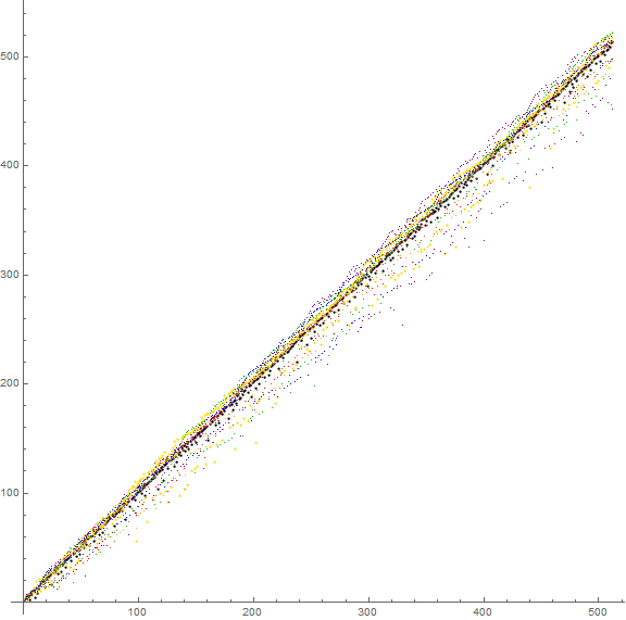
The familiar “diagonal” plot approximating a(b, n) = n pertains only to even bases; the odd bases plotted on same graph approximate a(b, n) = 2n.
Figure 8.2 is a plot of a(b, n) − n for even 2 ≤ b ≤ 16 in the same range with same color scheme:
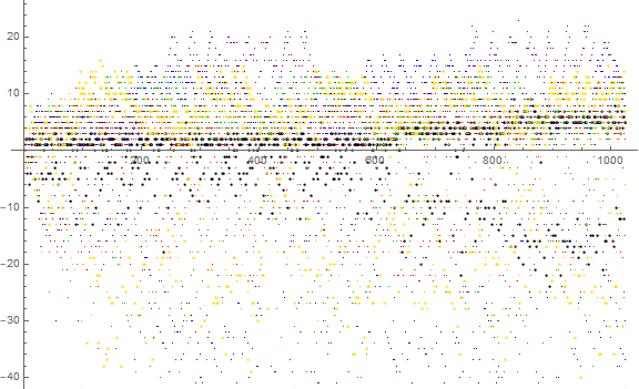
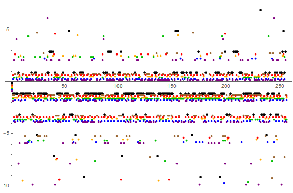
Odd b have a(b, n) approximate a(b, n) = 2n, with most values even negative or odd positive, the most common appearing to be −2. There is a much tighter spread among data in the plot a(b, n) − 2n, between −10 and +6 for bases 3 ≤ b ≤ 15 odd.
Figure 8.3 plots a(b, n) for odd 3 ≤ b ≤ 15 for 1 ≤ n ≤ 128 (for clarity). Black indicates base 3, with brown pertaining to 5, red pertaining to 7, orange to 9, green to 11, blue to 13, and purple to 15:
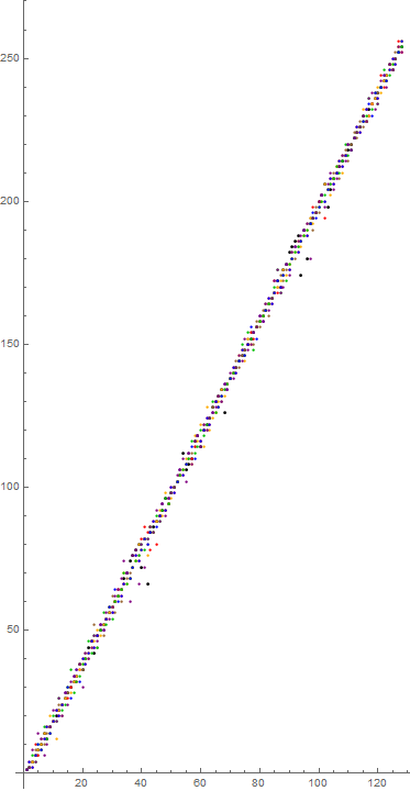
Figure 8.4 is a plot of a(b, n) − 2n for odd 3 ≤ b ≤ 15 and 1 ≤ n ≤ 256 with same color scheme:

Figure 8.5 is the same plot as Figure 8 but with data separated so that those pertaining to smaller bases appear above larger, spred within the vertical unit value so as to disambiguate coincident plots in Figure 8:
Topics to explore include the quasi-periodicity of a(n) exhibited in d(n).
This concludes our examination of OEIS A336893.
Nest[Append[#, Block[{k = 2, d = Map[IntegerDigits, #]},
While[Nand[FreeQ[#, k], GCD[FromDigits[#], Total[#]] &@
Flatten@ Append[d, IntegerDigits[k]] == 1], k++]; k]] &, {1}, 120]
Faster procedural code, with monitoring counter:
Monitor[Block[{s = 1, c = 1, a = {1}, f},
f[m_, n_] := m*10^(1 + Floor[Log10[n]]) + n;
Do[Block[{k = 2, d, t},
While[Nand[FreeQ[a, k],
GCD[Set[d, f[c, k]], Set[t, s + Total[IntegerDigits[k]]]] == 1], k++];
c = d; s = t; AppendTo[a, k]], {i, 2^12}]; a], i]
With[{b = 2}, Nest[Append[#, Block[{k = 2, d = Map[IntegerDigits[#, 2] &, #]},
While[Nand[FreeQ[#, k], GCD[FromDigits[#], Total[#]] &@
Flatten@ Append[d, IntegerDigits[k, 2]] == 1], k++]; k]] &, {1}, 120] ]
Code 2.1: Storing the result of Code 1.1 as variable a, we plot Figure 2.1:
ListPlot[MapIndexed[#1 - First[#2] &, a], ImageSize -> Large]
Code 3.1: Generate r(n), recordsetting indices of a(n):
r = Union@ FoldList[Max, a];
Code 3.2: Generate u(n), least unused k:
u = Block[{uu = 1, seq = a},
Array[Block[{}, While[! FreeQ[seq[[1 ;; #]], uu], uu++]; uu] &, Length@ seq]]
Code 3.3: Generate s(n), indices of records in a(n) − n:
s = With[{seq = MapIndexed[#1 - First@ #2 &, a]},
Map[FirstPosition[seq, #][[1]] &, Union@ FoldList[Max, seq]]]
Code 3.4: Generate t(n), recordsetting indices of a(n):
t = With[{seq = MapIndexed[First@ #2 - #1 &, a336893]},
Map[FirstPosition[seq, #][[1]] &, Union@FoldList[Max, seq]]]
Code 3.5: Generate z(n), recordsetting indices of a(n):
z = Position[Array[a[[#]] - # &, Length@ a], 0][[All, 1]];
Code 3.6: Generate Figure 3.2, plot a(n) for n ≤ 1000:
Block[{nn = 10^3, k}, k = Floor[nn/12]; Show[
ListPlot[
Array[Style[#,
Which[MemberQ[r, #], Darker[Red],
MemberQ[u, #], Darker[Blue],
True, Darker[Yellow]]] &@ a[[#]] &, nn],
ImageSize -> Large, PlotRange -> {{0, nn + k}, {0, nn + k}},
GridLines -> Automatic, AspectRatio -> 1, PlotStyle -> {LightGray, PointSize[Small]}],
ListPlot[
Array[If[FreeQ[s, #], -100,
Labeled[a[[#]], #, Before, LabelStyle -> Darker[Red]]] &, nn],
ImageSize -> Full, AspectRatio -> 1,
PlotRange -> {{0, nn + k}, {0, nn + k}}, Axes -> None,
PlotStyle -> {Red, PointSize[Large]}],
ListPlot[
Array[If[FreeQ[t, #], -100,
Labeled[a[[#]], #, After, LabelStyle -> Darker[Blue]]] &, nn],
ImageSize -> Full, AspectRatio -> 1,
PlotRange -> {{0, nn + k}, {0, nn + k}}, Axes -> None,
PlotStyle -> {Blue, PointSize[Large]}],
ListPlot[
Array[If[FreeQ[z, #], -100,
Callout[a[[#]], #, Above]] &, nn],
ImageSize -> Full,
AspectRatio -> 1, PlotRange -> {{0, nn + k}, {0, nn + k}},
Axes -> None, PlotStyle -> {Black, PointSize[Large]}] ] ]
Code 3.7: Generate Figure 3.3, plot a(n) − n for n ≤ 1000:
With[{nn = 10^3, j = 32, k = 84}, Show[
ListPlot[Array[a[[#]] - # &, nn], PlotRange -> {All, {-k, j}},
ScalingFunctions -> {"Log10", Automatic}, GridLines -> Automatic,
PlotStyle -> {LightGray, PointSize[Small]}],
ListPlot[Array[If[FreeQ[s, #], -k - 12,
Labeled[a[[#]] - #, #, LabelStyle -> Darker[Red]]] &, nn],
PlotRange -> {All, {-k, j}},
ScalingFunctions -> {"Log10", Automatic}, Axes -> None,
PlotStyle -> {Red, PointSize[Large]}],
ListPlot[
Array[If[FreeQ[z, #], -k - 12, a[[#]] - #] &, nn],
PlotRange -> {All, {-k, j}},
ScalingFunctions -> {"Log10", Automatic}, Axes -> None,
PlotStyle -> {Black, PointSize[Medium]}],
ListPlot[Array[
If[FreeQ[t, #], -k - 12,
Labeled[a[[#]] - #, #, LabelStyle -> Darker[Blue]]] &, nn],
PlotRange -> {All, {-k, j}},
ScalingFunctions -> {"Log10", Automatic}, Axes -> None,
PlotStyle -> {Blue, PointSize[Large]}], ImageSize -> Full]]
Nest[Append[#,
Block[{k = 3, d = Map[IntegerDigits, #]},
While[Nand[FreeQ[#, k], PrimeQ[FromDigits[#]] &@
Flatten@ Append[d, IntegerDigits[k]]], k += 2]; k]] &, {1}, 500]
Code 5.2: Generate the backstop v(n):
Monitor[Block[{s = 1, a, b, c = 1, f},
a = b = {1};
f[m_, n_] := m*10^(1 + Floor[Log10[n]]) + n;
Do[Block[{j, k, d, e, t}, j = k = 2;
While[Nand[FreeQ[a, j],
GCD[Set[d, f[c, j]], Set[t, s + Total[IntegerDigits[j]]]] == 1], j++];
While[
Nand[FreeQ[a, Set[e, (5 k + Mod[3 k + 2, 4] - 4)/2]],
PrimeQ@ f[c, e]], k++]; c = d; s = t; AppendTo[a, j];
AppendTo[b, e]], {i, 300}]; b], i]
g = With[{aa = Accumulate@ Map[Total@IntegerDigits[#] &, a336893]},
Array[GCD[s[[#]], aa[[#]]] &, Length@ s]];
Concerns sequences:
A002110: Primorials P(n) = products of the smallest n primes p.
A045572: Numbers k coprime to 10.
A083754: a(1) = 1; a(n) = least k in A045572 such that the grand concatenation a(1)..a(n) is prime.
A336893: Lexicographically earliest sequence of distinct positive terms such that the sum of digits of the first n terms is coprime to their concatenation; a(1) = 1.
Document Revision Record.
2020 0807 1700 Created. The document was written on Pensacola Beach during a vacation.
2020 0807 2000 a(n) to 10000 terms, b(n) to 4096 terms.
2020 0809 2300 b(n) corrected.
2020 0811 0730 Add figures 5 through 9.
2020 1111 2000 Expanded to include analysis of A336893 and news of a proof.