OEIS A338191

Written by Michael Thomas De Vlieger, St. Louis, Missouri, 2020 1015.

Abstract.

We examine 4 sequences directing the decimal digital root of the previous term to a nonzero digit d in the next term m that isn’t yet found in the sequence. The first sequence a(n) = OEIS A338191 applies d to the least digit of m, while b(n) = OEIS A248025 applies d to the least digit of m. We have studied a third sequence c(n) = OEIS A340138 that applies d to any digit in m in a separate paper. We also consider a version of c(n) that restricts m to only one instance of the digit d.

Introduction.

Let us consider 4 related self-referential sequences involving the decimal digital root d of the previous term governing the presence of the same digit d somewhere among those in a novel least term m not already in the sequence.

The digital root d(n) is the fixed point of the recursive summation of the decimal digits of n. Therefore, d(879) = 8 + 7 + 9 = 24; 2 + 4 = 6. We abbreviate this function in this work as n → d, thus, 879 → 6. We observe that the digital root results in a single decimal digit 0 ≤ d ≤ 9, however, we only obtain 0 when n = 0. Therefore:

d(0) = 0, d(n) = n mod 9 + [n mod 9 ≡ 0] (Iverson brackets).

The three sequences we consider directs the digit d to different positions in m. a(n) directs the digit d to the least digit of m; b(n) to the greatest digit of m, and c(n) to any digit of m.

Thus, we define the three sequences:

a(1) = 1; a(n) is the least m not already in a(n) that has the digital root d(a(n − 1)) as its least significant (i.e., last) digit. This sequence is OEIS draft A338191.

b(1) = 1; b(n) is the least m not already in b(n) that has the digital root d(b(n − 1)) as its most significant (i.e., first) digit. This sequence is OEIS A248025 by Éric Angelini.

c(1) = 0; c(n) is the least m not already in c(n) such that the digital root d(c(n − 1)) appears anywhere among the digits of m. We have studied this sequence at length in another paper; it appears here only for comparison with the first two.

s(1) = 0; s(n) is the least m not already in s(n) such that the digital root d(s(n − 1)) appears ONCE anywhere among the digits of m.

The notion of studying sequences a(n), b(n), and c(n) derives from David Sycamore.

The “root → least” sequence.

The sequence a(n) is rather simple, beginning:

1, 11, 2, 12, 3, 13, 4, 14, 5, 15, 6, 16, 7, 17, 8, 18, 9, 19, 21, 23, 25, 27, 29, 22, 24, 26, 28, 31, 34, 37, 41, 35, 38, 32, 45, 39, 33, 36, 49, 44, 48, 43, 47, 42, 46, 51, 56, 52, 57, 53, 58, 54, 59, 55, 61, 67, 64, 71, 68, 65, 62, 78, 66, 63, 69, 76, 74, 72, 79, 77, 75, 73, 81, 89, 88, 87, 86, 85, 84, 83, 82, 91, 101, 92, 102, 93, 103, 94, 104, 95, 105, 96, 106, 97, 107, 98, 108, 99, 109, 111, 113, 115, 117, 119, 112, 114, 116, 118, 121, 124, 127, 131, 125, 128, 122, 135, 129, 123, 126, 139, ...

(Generate per Code A)

The plot of a(n) is curious in that it involves a series of arrangements of terms in clusters of various patterns along a line with slope 10/9.

As a consequence of d(n) = 0 only for n = 0, m = 0 (mod 10) is prohibited. Therefore a(n) is not a permutation of the natural numbers, but contains all positive nonzero m indivisible by 10.

Figure A1: plot of a(n) for 1 ≤ n ≤ 324 (see Code A1):

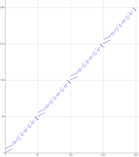
Graphing very many terms results in a line-like plot with slope 10/9, and it is clear that the sequence obeys some form of congruence recurrence.

Figure A2 labels the first 81 terms that seem to be repeated for n > 81, joining them for ease of interpretation and color-coding the dots according to a(n) mod 10, red = 1 through dark blue = 9, these extremes rendered larger than the other dots in order to aid in the examples that follow. (See Code A2)

Congruence Phases.

Let’s look at how the first terms are generated. We may write the function d(n) instead as “→” for brevity, separating the least novel m from d with a colon. Furthermore, we bold the number m not already in a(n) for clarity. Therefore, a(2) is derived from a(1) = 1 thus: 1 → 1: 11.

The sequence repeats 8 phases generally related to m mod 90 by decade (i.e., blocks of 10 along the y axis in Figure A2).

Phase 1 containing a(n) with 1 ≤ n ≤ 18 and involving 1 ≤ m mod 90 ≤ 19, begins as follows: 1 → 1: 11 → 2: 2 → 2: 12 → 3: 3, etc., therefore we have {1, 11, 2, 12, 3, 13, …, 19}, wherein we have each d twice in succession but incrementing d afterward. Therefore the first two decades are generated in tandem.

Phase 2 containing a(n) with 19 ≤ n ≤ 27 and involving m mod 90 in the 20s, results from 19 → 2, the third request for d = 2, so a(19) = 21. 21 → 3: 23 → 5: 25, etc. thus {21, 23, 25, 27, 29}, then 29 → 2: 22 → 4: 24, etc. thus {22, 24, 26, 28}.

Phase 3 contains a(n) with 28 ≤ n ≤ 36: 28 → 1: 31 → 4: 34 → 7: 37 → 1: 41 → 5: 35 → 8: 38 → 2: 32 → 5: 45 → 9: 39 → 3: 33 → 6: 36. This exhausts m mod 90 in the thirties. Generally, phases 3 | p involve m mod 90 = 10p + c(p + 1), with 0 ≤ c ≤ 1.

Phase 4 contains a(n) with 37 ≤ n ≤ 45 and begins with {41, 45} already used. 36 → 9: 49 → 4: 44 → 8: 48 → 3: 43 → 7: 47 → 2: 42 → 6: 46. This exhausts m mod 90 in the forties.

Phase 5 contains a(n) with 46 ≤ n ≤ 54: 46 → 1: 51 → 6: 56 → 2: 52, etc., thus {51, 56, 52, 57, 53, 58, 54, 59, 55}, exhausting m mod 90 in the fifties.

Phase 6 contains a(n) with 55 ≤ n ≤ 65: 55 → 1: 61 → 7: 67 → 4: 64 → 1: 71 → 8: 68 → 5: 65 → 2: 62 → 8: 78 → 6: 66 → 3: 63 → 9: 69. We have exhausted m mod 90 in the sixties.

Phase 7 contains a(n) with 66 ≤ n ≤ 72, begining with {71, 78} already used. 69 → 6: 76, etc., thus {76, 74, 72, 79, 77, 75, 73}, exhausting m mod 90 in the seventies.

Phase 8 is the last phase, ending with a(81): 73 → 1: 81 → 9: 89, etc., thus {81, 89, 88, ..., 83, 82}.

Recurrence Based on Congruences.

Having found a(1)..a(81), we may generate a(81k + j) = 90k + a( j), since a(82) = 91 → 1 and the next interval of 90 unused numbers are congruent to 0 < m < 90 (mod 9). By induction we see the sequence is infinite and contains all nonzero m (mod 90) that are indivisible by 10.

The sequence a(n) is easy to calculate for millions of terms.

The “root → most” sequence.

The sequence b(n) applies the digital root d to the first digit of a novel m not already in the sequence. It begins:

1, 10, 11, 2, 20, 21, 3, 30, 31, 4, 40, 41, 5, 50, 51, 6, 60, 61, 7, 70, 71, 8, 80, 81, 9, 90, 91, 12, 32, 52, 72, 92, 22, 42, 62, 82, 13, 43, 73, 14, 53, 83, 23, 54, 93, 33, 63, 94, 44, 84, 34, 74, 24, 64, 15, 65, 25, 75, 35, 85, 45, 95, 55, 16, 76, 46, 17, 86, 56, 26, 87, 66, 36, 96, 67, 47, 27, 97, 77, 57, 37, 18, 98, 88, 78, 68, 58, 48, 38, 28, 19, 100, 101, 29, 200, 201, 39, 300, 301, 49, 400, 401, 59, 500, 501, 69, 600, 601, 79, 700, 701, 89, 800, 801, 99, 900, 901, 102, 302, 502, ...

(Generate per Code B.)

Figure B1 is a plot of the first 3000 terms of b(n) that is logarithmic for b(n) but scalar for n (see Code B1):

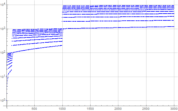
The plot manifests an exponential weaving pattern arrayed along lines that are 10^ek + j, such that e-digit indices n generally produce e-digit b(n). Instead of exhausting all the final digits of m, we consume the first digits, generally necessitating jumps approximately on the order of 10^ek between terms n with e digits.

Unlike a(n), we are permitted 10 | m in b(n), and since we accept no decimal number m that begins with a zero (d ≠ 0), b(n) is a permutation of the natural numbers.

There is a pattern in b(n) related to that seen in a(n) that recurs in an exponential way.

Figure B2 is a scalar plot of b(n) for 1 ≤ n ≤ 100, labeling the data and color-coding b(n) mod 9, with b(n) ≡ 0 (mod 9) in large red dots, through the spectrum to blue for 8 (mod 9) in order to aid the examples (see Code B2).

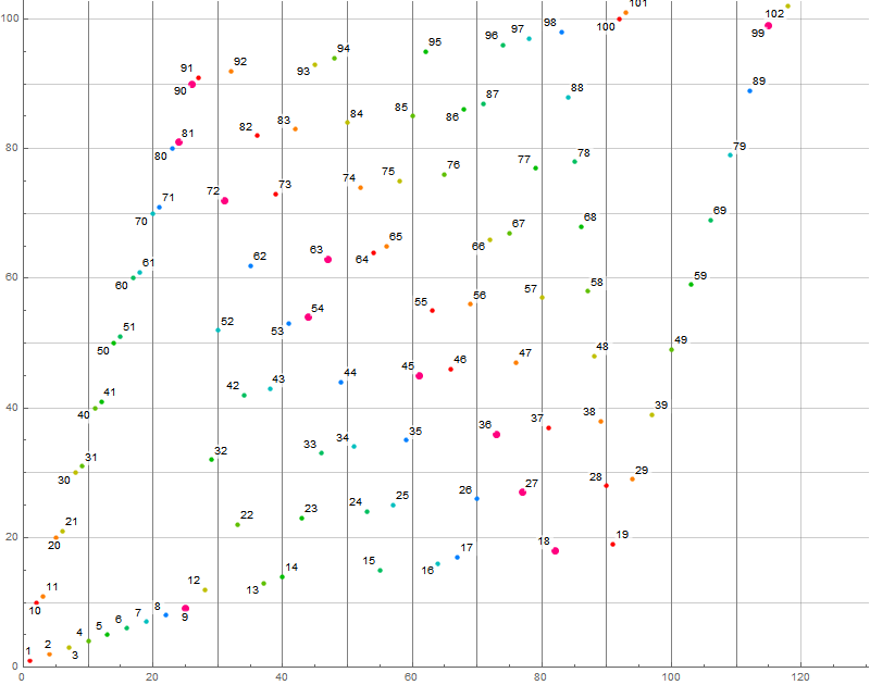
We see, in aggregate, that we exhaust numbers m that start with digit d in a strictly increasing way as n increases, interrupted as necessary when d takes other values, until we exhaust all the numbers j between 10^ek and 10^e(k + 1).

Transition between Exponential Phases.

Also in general, but not visible in Figure B2, there is a transition zone between phases featuring m with e digits, beginning with an introductory intercalation of 10^ek − 1 with the consecutive pair 10^{(e + 1)}k and 10^{(e + 1)}k + 1 for 1 ≤ k ≤ 9. This exhausts all the m in the phase e (i.e., all the e-digit m, in other words, all m < 10^{(e + 1)}). As a by-product, all 10^{(e + 1)}k + j for 1 ≤ k ≤ 9 and 0 ≤ j ≤ 1 are expended, which are m in phase (e + 1).

Congruence Phases.

Phase 1 is purely the transition between e = 1 and e = 2 (i.e., m with e digits). We begin with 1 → 1: 10 → 1: 11 → 2: 2 → 2: 21 → 3: 3, etc. through 90 → 9: 91. This exhausts phase e = 1, i.e., all the single-digit m. As a by-product, we have already generated the double-digit m that end in 0 and 1. Generally speaking, this is all 10k + j for 1 ≤ k ≤ 9 and 0 ≤ j ≤ 1, i.e., {10, 11, 20, 21, 30, 31, …, 91}.

Phase 2 consumes all m for e = 2, and includes the transition to phase 3 as described generally.We see in phase 2 that the units digit imparts influence on the pattern through digital root. Instead of decades, we are running through the numbers j, the range 1 ≤ k ≤ 9 prepended to them as n increases.

Therefore we have 12 → 3: 32, thus {12, 32, 52, 72, 92}, then 92 → 2: 22, thus {22, 42, 62, 82}; we complete the two-digit numbers m that end in j = 2.

We move from 82 → 1: 13 → 4: 43, thus {13, 43, 73, 14, 53, 83, 23, 54, 93, 33, 63, 94, 44, 84, 24, 64}, mixing j = 3 and j = 4.

The sequence passes through j = 5 thus: {15, 65, 25, 75, 35, 85, 45, 95, 55}.

We see j = 6 and j = 7 intermixed akin to j = 3 and j = 4: {16, 76, 46, 17, 86, 56, 26, 87, 66, 36, 96, 67, 47, 27, 97, 77, 57, 37}.

Finally, we move through j = 8 from 37 → 1: 18 with k decrementing from 9: {18, 98, 88, 78, 68, 58, 48, 38, 28}. The transformation 28 → 1: 100 leads us to the transition as described above.

Generally in subsequent phases, the digital root k + j (mod 9), with residue 0 read instead as 9, cycles through the 10^{(e − 1)} numbers j in a similar fashion. Since gcd(9, 10) = 1, the residues cover any phase e, and we have a permutation of the natural numbers in b(n).

There might be an efficient way to generate b(n) based on congruences without a self-referential function, i.e., checking whether m already appears in b(n). This remains to be done.

The “root → any” or “frayed rope” sequence.

The sequence c(n) = A340138(n) applies the digital root d to any digit of a novel m not already in the sequence. (Generate it using Code C.) It begins:

0, 10, 1, 11, 2, 12, 3, 13, 4, 14, 5, 15, 6, 16, 7, 17, 8, 18, 9, 19, 21, 23, 25, 27, 29, 20, 22, 24, 26, 28, 31, 34, 37, 41, 35, 38, 32, 45, 39, 30, 33, 36, 49, 40, 42, 46, 51, 56, 52, 47, 62, 48, 43, 57, 53, 58, 44, 68, 50, 54, 59, 55, 61, 67, 64, 71, 78, 60, 63, 69, 65, 72, 79, 70, 73, 81, 89, 80, 82, 91, 100, 101, 92, 102, 83, 112, 74, 120, 93, 103, 84, 113, 75, 123, 66, 130, 94, 104, 85, 114, 76, 124, 77, 95, 105, 86, 115, 87, 96, 106, 97, 107, 88, 117, 90, 98, 108, 99, 109, 110, ...

Figure C1 is a plot of the first 1000 terms of c(n) (see Code C1):

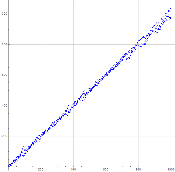
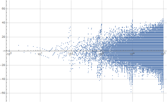
The plot is more complex than those of a(n) or b(n), but tightly clusters around a line from origin with slope 1. Because of this, we can examine c(n) more thoroughly by running a log plot of c(n) − n.

Figure C2 is log plot of c(n) − n for 1 ≤ n ≤ 100000 (see Code C2):

We examine this sequence at length in its own essay, on account of its relative complexity.

The “root → any-and-once” sequence.

The sequence s(n) applies the digital root d to any single digit of a novel m not already in the sequence. (Use Code S to generate.)

s(1) = 0; s(n + 1) is the lexicographically earliest m such that d = digital root of a(n) appears once among its decimal digits.

It begins:

0, 10, 1, 12, 3, 13, 4, 14, 5, 15, 6, 16, 7, 17, 8, 18, 9, 19, 21, 23, 25, 27, 29, 2, 20, 24, 26, 28, 31, 34, 37, 41, 35, 38, 32, 45, 39, 30, 36, 49, 40, 42, 46, 51, 56, 52, 47, 62, 48, 43, 57, 53, 58, 54, 59, 50, 65, 72, 69, 60, 61, 67, 64, 71, 68, 75, 63, 79, 70, 73, 81, 89, 78, 76, 74, 82, 91, 100, 102, 83, 92, 112, 84, 93, 103, 94, 104, 85, 114, 86, 95, 105, 96, 106, 87, 116, 80, 98, 108, 90, 97, 107, 118, 109, 120, 113, 115, 117, 119, 121, 124, 127, 122, 125, 128, 123, 126, 129, 130, 134, ...

This variant of the “root → any” sequence c(n) is more constrained than c(n); it does not cluster around a line with slope 1. Instead s(n) has slope slightly greater than 1.

Numbers m more than single-digit that are repdigits or solely contain more than 1 of its constituent digits and any zeros are not in s(n). The smallest of these are listed in x(n) below (see Code X).

11, 22, 33, 44, 55, 66, 77, 88, 99, 101, 110, 111, 202, 220, 222, 303, 330, 333, 404, 440, 444, 505, 550, 555, 606, 660, 666, 707, 770, 777, 808, 880, 888, 909, 990, 999, 1001, 1010, 1011, 1100, 1101, 1110, 1111, 1122, 1133, 1144, 1155, 1166, 1177, 1188, 1199, 1212, 1221, 1313, 1331, 1414, 1441, 1515, 1551, 1616, 1661, 1717, 1771, 1818, 1881, 1919, 1991, 2002, 2020, ...

For this reason we see that the plot of s(n) actually follows a slightly curved trajectory. Taking the mean of s(n)/n for n < {100, 1000, 10000} we have approximately 1.10012, 1.05169, and 1.03534 respectively.

Figure S1 is a plot of the first 1000 terms of s(n) in prominent blue, vs. the plot of the first 1000 terms of c(n) in light pink (see Code S1):

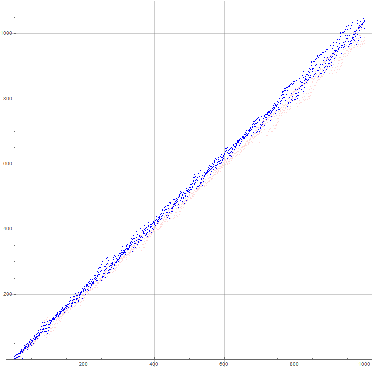
Figure S2 is a plot of s(n) − (10000/9685)n for 1 < n < 10000, akin to Figure C2, the ratio 10000/9685 accounting for the 315 terms in x(n) that are less than or equal to 10000 (see Code S2):

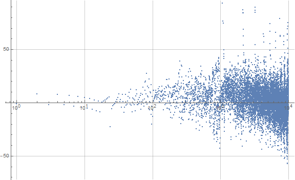
The point of Figure S2 is to show that dynamics similar to c(n) are at work in s(n), despite the distortion in the latter sequence.

One could devise similar sequences in alternate bases, particularly binary, where the digital root is replaced by the binary weight of the previous term. This will be the subject of study of a coming paper.

This concludes our examination of sequences directing the decimal digital root of the previous term to a nonzero digit d in the next term m that isn’t yet found in the sequence.

Appendix:

Code A: Generate a(n) and store it in variable a:

a = With[{s = Nest[Append[#, Block[{k = 1,
  r = Mod[#[[-1]], 9] + 9 Boole[Mod[#[[-1]], 9] == 0]},
  While[Nand[FreeQ[#, k], Mod[k, 10] == r], k++]; k]] &, {1}, 9^2]},
  Array[If[#2 == 0, 90 #1 - 8, 90 #1 + s[[#2]] ] & @@
    QuotientRemainder[#, 81] &, 10^3]];

Code A1: Plot a(n) per Figure A1:

With[{lo = 1, hi = 4*9^2, max = 12, k = 1, r = 1},
  ListPlot[a[[lo ;; hi]], ImageSize -> Large,
  AspectRatio -> Automatic, PlotStyle -> {Blue, PointSize[Small]},
  GridLines -> {9^2*Range[lo - 1, Floor[hi/9]], 90*Range[lo, Floor[hi/9]]},
  Ticks -> {9^2*Range[lo - 1, Floor[hi/9]], 90*Range[lo, Floor[hi/9]]}]]

Code A2: Plot a(n) per Figure A2:

With[{lo = 1, hi = 9^2 + 1, max = 12, k = 1, r = 1},
  Show[{ListPlot[ConstantArray[-100, lo - 1]~Join~
    MapIndexed[
      Labeled[Style[#2, Hue[(#3 - k)/max, 1, 1 - Boole[FreeQ[{0, 1, 2, 8}, #3]]/4],
        PointSize@ If[MemberQ[{1, 9}, #3], Large, Medium]], #4] & @@
      {#2, #1, Mod[#1, 10], #}& @@ {#1, First[#2] + lo} &, a[[lo ;; hi]]],
      ImageSize -> 800, Joined -> True, AspectRatio -> Automatic,
      PlotRange -> {{lo - 1, hi}, {lo - 1, 10 hi/9}},
      GridLines -> {9 Range[lo, Floor[hi/9]], 10 Range[lo - 1, Floor[hi/9]]},
      Ticks -> {9 Range[lo - 1, Floor[hi/9]], 10 Range[lo, Floor[hi/9]]},
      PlotStyle -> {LightGray, Thin, PointSize[Tiny]}]},
    Graphics[{Pink, Dashed, Line[{{lo, lo}, {hi, 10 hi/9}}]}]]]

Code B: Generate b(n) and store it in variable b:

b = Nest[Append[#,
  Block[{k = 1, r = Mod[#[[-1]], 9] + 9 Boole[Mod[#[[-1]], 9] == 0]},
    While[Nand[FreeQ[#, k], IntegerDigits[k][[1]] == r], k++]; k]] &, {1}, 10^4]

Code B1: Plot b(n) per Figure B1:

ListPlot[b[[1 ;; 3*10^3]], ImageSize -> Large, ScalingFunctions -> "Log10",
  GridLines -> Automatic, PlotStyle -> {Blue, PointSize[Small]}]

Code B2: Plot b(n) per Figure B2:

With[{lo = 1, hi = 120, max = 12, k = 1, r = 1},
  ListPlot[ConstantArray[-100, lo - 1]~Join~
    MapIndexed[
      Labeled[Style[#2, Hue[(#3 - k)/max, 1, 1 - Boole[FreeQ[{0, 1, 2, 8}, #3]]/4],
        PointSize@ If[#3 == 0, Large, Medium]], #4] & @@
        {#2, #1, Mod[b[[#2 - 1]], 9], #1} & @@ {#1, First[#2] + lo} &, b[[lo ;; hi]]],
  ImageSize -> 800, AspectRatio -> Automatic,
  PlotRange -> {{lo - 1, hi}, {lo - 1, 10 hi/12}},
  GridLines -> {10 Floor[Range[lo - 1, hi]/10], 10 Range[lo - 1, Floor[hi/12]]},
  Ticks -> {10 Floor[Range[lo - 1, hi]/10], 10 Floor[hi/12]},
  PlotStyle -> {LightGray, Thin, PointSize[Tiny]}] ]]

Code C: Generate c(n) and store it in variable c:

c = Nest[Append[#, Block[{k = 1,
  r = Mod[#[[-1]], 9] + 9 Boole[Mod[#[[-1]], 9] == 0]},
  While[Nand[FreeQ[#, k], ! FreeQ[IntegerDigits[k], r]], k++]; k]] & @@
    {#, Length@ #} &, {0, 10}, 10^2]

Code C1: Plot c(n) per Figure C1:

ListPlot[c[[1 ;; 10^3]], ImageSize -> Full, AspectRatio -> 1,
  GridLines -> Automatic, PlotStyle -> Directive[Blue, PointSize[Small] ] ] ]

Code C2: Plot c(n) similar to Figure C2:

ListPlot[MapIndexed[#1 - First[#2] &, c],
  ImageSize -> Large, PlotRange -> {All, {-72, 72}},
  ScalingFunctions -> {"Log10", Automatic}, GridLines -> Automatic,
  PlotStyle -> PointSize[Small]]

Code S: Generate s(n) and store it in variable s:

s = Nest[Append[#,
  Block[{k = 1, r = Mod[#[[-1]], 9] + 9 Boole[Mod[#[[-1]], 9] == 0]},
  While[Nand[FreeQ[#, k], DigitCount[k, 10, r] == 1], k++]; k]] & @@
    {#, Length@ #} &, {0, 10}, 10^2]

Code S1: Plot s(n) per Figure S1:

ListPlot[{c, s}, ImageSize -> Full, AspectRatio -> 1, GridLines -> Automatic,
  PlotStyle -> {Directive[LightRed, PointSize[Small]],
  Directive[Blue, PointSize[Small]]}]

Code S2: Plot s(n) similar to Figure S2:

ListPlot[MapIndexed[#1 - (10000/9685) First[#2] &, s[[1 ;; 10^4]]],
  ImageSize -> Large, PlotRange -> {All, {-72, 96}},
  ScalingFunctions -> {"Log10", Automatic}, GridLines -> Automatic,
  PlotStyle -> PointSize[Small]]

Code X: Generate x(n), the numbers not in s(n):

Select[Range[10^4], AllTrue[DeleteCases[Most@ DigitCount[#], 0], # > 1 &] &]

Concerns OEIS sequences:

A248025 Find d(a(n − 1)) in most significant rank of unique m.
A338191 Find d(a(n − 1)) in least significant rank of unique m.
A340138 Find d(a(n − 1)) anywhere within the decimal expansion of unique m.

Document Revision Record.

2020 1016 1230 Created.
2020 1119 1900 Update.
2021 0122 0715 Add links to A340138.