OEIS A341679.
A sequence of Scott R. Shannon.
Written by Michael Thomas De Vlieger, St. Louis, Missouri, 2021 0302.
Abstract.
An examination of the behavior of Shannon’s sequence OEIS A341679.
Introduction.
We define a self-referential divisor-seeking sequence a(n) = A341679(n) as follows:
a(1) = 1; a(n) = n/d where d is the most recent d | n in a.
We thus define m = a(n), therefore m × d = n. The sequence a begins:
1, 2, 3, 2, 5, 3, 7, 4, 3, 2, 11, 6, 13, 7, 5, 8, 17, 3, 19, 4, 7, 2, 23, 12, 5, 13, 9, 14, 29, 6, 31, 16, 11, 17, 7, 6, 37, 19, 3, 8, 41, 14, 43, 4, 15, 2, 47, 24, 7, 25, 17, 26, 53, 27, 5, 8, 19, 29, 59, 12, 61, 31, 9, 8, 13, 33, 67, 4, 23, 14, 71, 18, 73, 37, 15, 19, 11, 6, 79, 20, 9, 41, 83, ...
Code 1 generates the sequence in a syntactically concise way, however Code 2 memoizes the most recent index of m and is thus faster. We have obtained 220 terms.
We may also define an auxiliary sequence b(n) = d = a(n)/n. This sequence begins:
1, 1, 1, 2, 1, 2, 1, 2, 3, 5, 1, 2, 1, 2, 3, 2, 1, 6, 1, 5, 3, 11, 1, 2, 5, 2, 3, 2, 1, 5, 1, 2, 3, 2, 5, 6, 1, 2, 13, 5, 1, 3, 1, 11, 3, 23, 1, 2, 7, 2, 3, 2, 1, 2, 11, 7, 3, 2, 1, 5, 1, 2, 7, 8, 5, 2, 1, 17, 3, 5, 1, 4, 1, 2, 5, 4, 7, 13, 1, 4, 9, 2, 1, 6, 5, 2, 29, 11, 1, 3, 13, 23, ...
Observe that b(n) = 1 for n = 1 and n prime. Conversely, a(n) = n for n = 1 and n prime. Clearly, 1, the empty product, is given; it is the only available divisor for any p, since p is coprime to all smaller n, i.e., gcd(p, n) = 1 for all n < p. As a consequence of a(p) = p, a(1) = 1 is the only appearance of 1 in the sequence.
Furthermore, b(pε ) = pk, 1 ≤ k ≤ ε, for all perfect prime powers pε, hence a(pε ) = p(ε − k), since pk × p(ε − k) = pε.
As regards n = k², we sometimes have a(n) = k = b(n). It is certain that a(p²) = p = b(p²). Hence we might talk of the appearance of p in sequence a for n = p and n = p² as “trivial”.
Records in a are 1 and the primes and thus, the sequence has the bound a(n) ≤ n. There can be no m > prime(π(p)), since m = p prime enters first at a(p). The minimum is a(1) = 1, while local minima appear for m = 2 at certain even n.
The sequences a and b are multiplicatively complementary therefore the records in one become the local minima in the other.
Figure 1 is an annotated scatterplot of a(n) for 1 ≤ n ≤ 64. The color function relates to b(n) = a(n)/n. Hence, red pertains to b(n) = 1, orange to b(n) = 2, etc.
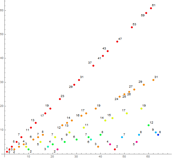
In Figure 1, the records appear in red. The minimum a(1) = 1 and the local minima m = 2 are simply labeled such. We see that the terms m occupy streets or trajectories d along rays with origin (d, 1) slope = 1/d = m/n. Hence we attain a rectified, coherent picture of all trajectories d with slope 1 through use of a log-log plot.
Figure 2 is a log-log scatterplot of a(n) for 1 ≤ n ≤ 4096, with a color function as to d.
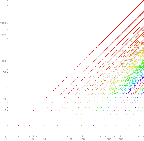
Examining each trajectory d, we see an interesting irregular “compression-rarefaction” or “dashing” behavior as n increases. This behavior seems more “solid” for d = 1 and d prime, but exponentially intermittent for composite d.
Unfolding the exponential plot of a(n).
We can “unfold” Figure 2 though a scalar scatterplot of b(n).
Figure 3 is a scatterplot of b(n) for 1 ≤ n ≤ 4096, with composite d in blue, otherwise red.
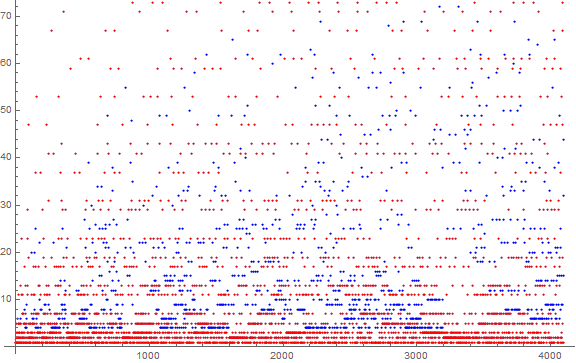
The “solidity” of the trajectories d need to take into account the pitch d, since we only have d | n. Therefore a different sort of graph need be made. The graph procedure involves the following.
First, we glean positions i of d in sequence b and store it in datum D. We map the function f(x) = i/d (which yields the integer m) across datum D. At some point, due to insufficient data, a null D materializes which we shall use as a y-axis delimiter or dmax. Using the greatest term mmax in datum Dmax pertaining to dmax, we then trim values m > mmax in data D < Dmax so as to obtain addresses bounded on the x-axis by mmax. Next, we presume all m absent from D to have value 0, and all m in D to have value 1, so as to generate a bitstring. Together, all the bitstrings D comprise a raster. By this method we have ironed out the effects of the pitch d.
The resultant graph situates the trajectories d along the y-axis, and the m in each trajectory along the x-axis. Hence, for n = dm, we have a term at the coordinate (m, d) for a particular pair of nontrivial complementary divisors for composite n. The pattern of appearances of m in any given trajectory d appear in columns, and the scale adjusted “density” of trajectory d is made evident along the rows of the graph. This graph “unfolds” the standard scalar plot of a(n).
Figure 4 is an annotated graph that plots the circle n = md at coordinate (m, d), with the origin at the lower left corner. The x-axis represents m = a(n) and the y-axis d =n/a(n). The numbers n appear in the circle. If both d and m are noncomposite, the circle is black, if d is prime, the circle is red, otherwise the circle is colored blue. The light gray gridlines are struck at each prime in both axes, and 1 in the y-axis.
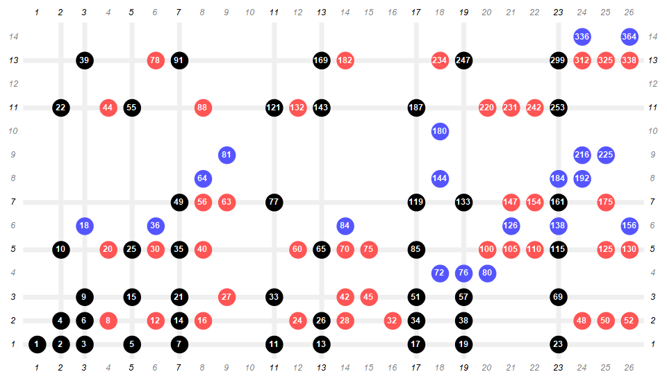
Hence we see, as is obvious, that only certain products md → a(md) so as to construct a permutation of the natural numbers per the definition of a.
Figure 5 is a graph that plots n = md at coordinate (m, d), with the origin at the lower left corner. The x-axis represents m = a(n) and the y-axis d = n/a(n). If both d and m are noncomposite, the dot is black, if d is prime, the dot is red, otherwise the dot is colored blue. The light gray gridlines are struck at each prime in both axes, and 1 in the y-axis. (Click here for a larger view)
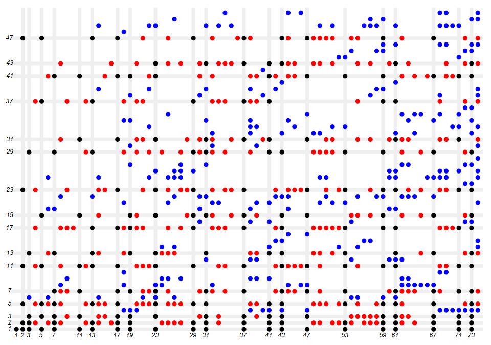
This Figure 5 suggests that we are likely to see a(pq) = q, with primes p < q, when p is small.
Figure 6 is a graph that plots n = md at coordinate (m, d), with the origin at the lower left corner, using the 1048576-term dataset and releasing the constraints governed by unpopulated data D. Instead, we have selected a sample where mmax = dmax = 960, an arbitrary limit.
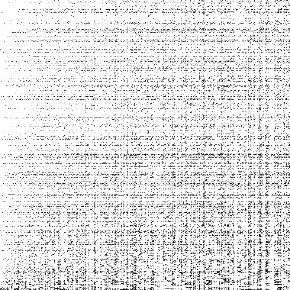
The graph looks like a scuffed tartan pattern. To be more precise, it seems that (m, d) is likely to be populated if m and d prime, and if a nearby coordinate closer toward the origin has appeared. There appears to be a slight bias toward the lower right half of the graph, meaning, in favor of gpf(n) = a(n), where gpf(n) is the greatest prime divisor of n.
Assessing the intensity of the compression of the trajectory d.
We define a function s(n) that, given input d = b(n), reports the number ℓ of instances of d in b(n) for 1 ≤ k ≤ n. The sequence s begins:
1, 2, 3, 1, 4, 2, 5, 3, 1, 1, 6, 4, 7, 5, 2, 6, 8, 1, 9, 2, 3, 1, 10, 7, 3, 8, 4, 9, 11, 4, 12, 10, 5, 11, 5, 2, 13, 12, 1, 6, 14, 6, 15, 2, 7, 1, 16, 13, 1, 14, 8, 15, 17, 16, 3, 2, 9, 17, 18, 7, 19, 18, 3, 1, ...
Figure 7 is a scatterplot of s(n) for 1 ≤ n ≤ 256, with a color function and label reporting b(n).
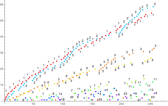
In Figure 7, each d = n/a(n) has a trajectory that has ℓ inrement for each occasion of d in b as n increases. We can see the trajectory of d = 2 surpass that of d = 1 only to slow down and fall under d = 1. The trajectory of d represents the “intensity” of compression of the same in the scatterplot of sequence a.
Particularly, we see the trajectory of d = 2 commence an acceleration phase at a(96) = 48. Thereafter, d = 2 | n for even n occurs intensively, due to the inavailability of larger divisors for the even indices 96 ≤ n ≤ 118. The cycle appears to be broken by highly composite n = 120, a(120) = 6. Meanwhile the trajectories of d = 3 and d = 5 appear to tricke through unabated. We see in sequence a that relatively large divisors m enter the sequence, therefore d tends to be small and prime, and the occasion of composite d is suppressed.
Figure 8 is a scatterplot of s(n) for 1 ≤ n ≤ 65536.
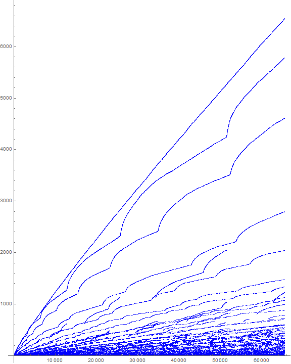
Figure 8 demonstrates, in general, the apparent exponentially-scaled cycling or throttling of the trajectories.
Figure 9 is a log-log scatterplot of s(n) for 1 ≤ n ≤ 16384, where the color function codes d = 1 blue, prime d red, and composite d black.
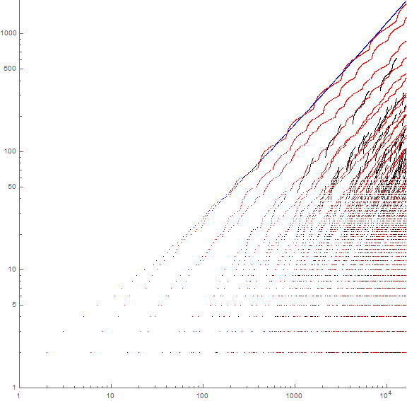
Work in progress.
Appendix:
Code 1: Generate a(n) (syntactically simpler, via reverse counter):
Block[{a = {1}, k},
Do[k = 1; While[Mod[i, a[[-k]]] != 0, k++];
AppendTo[a, i/a[[-k]] ], {i, 2, 83}]; a]
Code 2: Generate a(n) (memoize the last index n of m):
Block[{a = {1}, c, k}, c[1] = 1;
Monitor[Do[AppendTo[a, Set[k, i/
MaximalBy[Map[If[! IntegerQ@ c[#], {#, 0}, {#, c[#]}] &,
Divisors[i]], Last][[1, 1]] ]];
c[k] = i , {i, 2, 2^16}], i]; a]]
Concerns OEIS sequences:
A341679: a(n).
Document Revision Record.
2021 0302 2000 Created.
2021 0303 1645 Draft 1.