The Sandwich Sequence
OEIS A350359, a sequence by David Sycamore.
T
his page written by Michael Thomas De Vlieger, St. Louis, Missouri, 2021 1226.
Abstract.
Analysis of A350359, a sequence restrictive of equality and coprimality, bookended by terms that must be coprime to the middle and currently generated term. The sequence exhibits behavior akin to A064413, A098550, and A347113. The sequence appears to be a permutation of natural numbers. The aim of this work is to explain features of the scatterplot.
Introduction.
Let s(n) = n for 1 ≤ n ≤ 3, let a = s(n−3), b = s(n−2), and c = s(n−1). Let s(n) be the least k not already in s such that gcd(a,d) = gcd(c,d) = 1, but gcd(b,d) > 1. This is tantamount to the recursive mappings of the following function f(x):
{fn( a, b, c) → d : s(n−2) → a ∧ s(n−1) → b ∧ s(n) → c :
k ∉ s(1..n) ∧ (a, d) = (c, d) = 1 ∧ (b, d) > 1}
where s(1..3) = 1..3.
The first terms of s follow:
1, 2, 3, 4, 9, 8, 15, 14, 5, 7, 25, 21, 10, 27, 16, 33, 20, 11, 26, 77, 6, 35, 12, 49, 18, 91, 22, 13, 24, 65, 28, 55, 32, 45, 34, 39, 17, 57, 68, 19, 40, 133, 30, 119, 36, 161, 38, 23, 44, 69, 50, 51, 52, 63, 46, 75, 58, 81, 29, 93, 116, 31, 56, 155, 42, 85, 48, 95, 54, 115, 62, 125, 64, 105, 74, 87, 37, 99, 148, 117, 70, 123, 76, 41, 80, 287, 60, 203, 66, 217, 72, 175, 78, 145, 82, 185, 84, 215, 88, 43, 92, 129, 94, 111, 47, 135, 188, 147, 86, 153, 100, 141, 98, 159, 104, 53, 110, 371, 90, 259, ...
Code 1 generates the sequence efficiently. Through an extensible version of Code 1, we have obtained a dataset of 220 terms.
Consequences of definition includes forbidden equality, while we restrict a and c to coprimality with d, yet b and d have coprimality forbidden. Odd numbers may be adjacent but even numbers cannot be adjacent; generally if prime q | s(n), then q is coprime to s(n±1). If q is small, especially if q = 2, then often, q | s(n±2).
The sequence is lexically earliest, hence there are 3 seeds {1, 2, 3} drawn sequentially into input. As a consequence, the sequence forces prime d | b thus b > d and prime b | d thus b < d. Hence s(n−2) = kp and s(n+2) = mp for s(n) = p prime, with k ⊥ s(n−1) ∧ m ⊥ s(n+1).
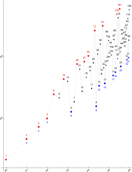
Figure 1.1: Annotated log-log scatterplot of s(n) for 1 ≤ n ≤ 32, showing records in red and minima in blue. Code 7 generates this plot.
Auxiliary sequences.
Define sequence d(n) = gcd(b,d); this sequence begins:
1, 2, 3, 4, 3, 2, 5, 7, 5, 7, 5, 3, 2, 3, 4, 11, 2, 11, 2, 7, 6, 7, 6, 7, 2, 13, 2, 13, 4, 5, 4, 5, 2, 3, 17, 3, 17, 19, 4, 19, 10, 7, 6, 7, 2, 23, 2, 23, 2, 3, 2, 3, 2, 3, 2, 3, 29, 3, 29, 31, 4, 31, 14, 5, 6, 5, 6, 5, 2, 5, 2, 5, 2, 3, 37, 3, 37, 9, 2, 3, 2, 41, 4, 41, 20, 7, 6, 7, 6, 7, 6, 5, 2, 5, 2, 5, 4, 43, 4, 43, 2, 3, 47, 3, 47, 3, 2, 3, 2, 3, 2, 3, 2, 53, 2, 53, 10, 7, 6, 7, ...
Records r begin as follows:
1, 2, 3, 4, 9, 15, 25, 27, 33, 77, 91, 133, 161, 287, 371, 657, 749, 1017, 1251, 1337, 2007, 2763, 3141, 3897, 5193, 5579, 6349, 6503, 6559, 6769, 8973, 11619, 11943, 12061, 12313, 13993, 18261, 21699, 23931, 29709, 35147, 46017, 46076, 46196, 46204, 46316, 46348, ...
Minima s appear as follows:
1, 2, 3, 4, 5, 6, 12, 13, 17, 19, 23, 29, 31, 37, 41, 43, 47, 53, 59, 61, 67, 71, 73, 79, 83, 89, 97, 101, 103, 107, 109, 113, 127, 131, 137, 139, 149, 151, 157, 163, 167, 173, 179, 181, 191, 193, 197, 199, 211, 223, 227, 229, 233, 239, 241, 251, 257, 263, 269, 271, 277, 281, 283, 293, 307, 311, 313, 317, 331, 337, 347, 349, 353, 359, 367, 373, 379, 383, 389, ...
Let the characteristic sequence of parity, P(n) = s(n) mod 2:
1, 0, 1, 0, 1, 0, 1, 0, 1, 1, 1, 1, 0, 1, 0, 1, 0, 1, 0, 1, 0, 1, 0, 1, 0, 1, 0, 1, 0, 1, 0, 1, 0, 1, 0, 1, 1, 1, 0, 1, 0, 1, 0, 1, 0, 1, 0, 1, 0, 1, 0, 1, 0, 1, 0, 1, 0, 1, 1, 1, 0, 1, 0, 1, 0, 1, 0, 1, 0, 1, 0, 1, 0, 1, 0, 1, 1, 1, 0, 1, 0, 1, 0, 1, 0, 1, 0, 1, 0, 1, 0, 1, 0, 1, 0, 1, 0, 1, 0, 1, 0, 1, 0, 1, 1, 1, 0, 1, 0, 1, 0, 1, 0, 1, 0, 1, 0, 1, 0, 1, ...
Code 2 provides Mathematica script that generate these auxiliary sequences and others.
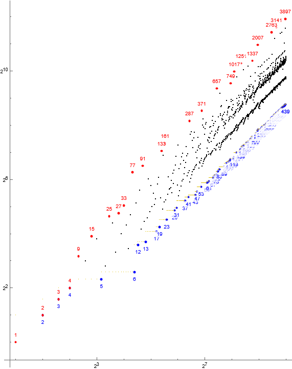
Figure 1.2: Log-log scatterplot of s(n) for 1 ≤ n ≤ 210 showing maxima r in red and minima t in blue. The golden line indicates the least unused number u.
Parity.
An important consequence of the sequence definition is that runs of odd terms are not prohibited, but there cannot be even runs. Generally, if q is prime, then q may not divide adjacent terms. The spacing of even terms is in {2, 4, 5}, the last rarely, while that of odd terms is {1, 2}, the former occasionally.
Odd run lengths ℓ are either 1, 3, or 4. The apparent limitation is understandable given the impetus for even terms to appear every other term. Run lengths 3 ≤ ℓ ≤ 4 that start at s(n) associate with prime s(n+1).
Even squarefree semiprimes.
Almost all even squarefree semiprime 2p = s(n) precipitates an extended odd run length ℓ > 1 by observation.
Since s(n) is even, it is flanked by s(n±1) divisible by any primes q except 2 and p, hence p may appear unless there is an unused u < p : 2 | u ∨ p | u. Normally this is p itself, however, there is a special class of 2p early in the sequence that appear well after p has already appeared. For these s(n) = 2p, we have s(n+1) odd and 2 | s(n), hence ℓ = 1. Let us call these “late” even squarefree semiprimes. There appear to be a finite number of such given a dataset of 220 terms; we list their indices n here:
13, 21, 27, 47, 55, 71, 95, 109, 125, 182, 198, 228, 254, 276, 296, 328, 357, 395, 419, 445, 466, 525, 531, 554, 594, 629, 663, 711, 729, 778, 808, 889, 921, 985, 1007, 1019, 1045, 1069, 1089, 1169, 1207, 1255, 1331, 1395, 1421, 1437, 1480, 1512, 1610, 1664, 1699, 1754, 1852, 1895, 1913, 1983, 2096, 2148, 2164, 2238, 2292, 2443, 2465, 2534, 2544, 2610, 2748, 2816, 2848, 2996, 3033, 3083, 3290, 3333, 3364, 3402, 3417, 3433, 3639, 3719, 3744, 3988, 4075, 4343, 4471, 4519, 4583, 4632, 4704, 4980, 4998, 5183, 5317, 5351, 5549, 5586, 5914, 6011, 6158, 6234, 6263, 6365, 6520, 6891, 7017, 7067, 7675, 7699, 7719, 7868, 8564, 9039, 9138, 9160, 9496, 9637, 9867, 9929, 9979, 11698, 11891, 13686
Early effect on primorials.
The case of s(19) = 26 is special and is linked with another special case, s(21) = 6.
Since 6 = 2 × 3, the smallest primes, it has a slight totient. Both facts conspire to delay its entry such that when 2 | s(n−2), 3 | s(n−3) ∧ 3 | s(n−1). The first break comes s(19) = 26. Since 2 | u, we have s(21) = 6 instead of 13. This is the only exception to the general pattern of kp → p : p = lpf(kp) in the sequence on account of severely minimized totient of 6.
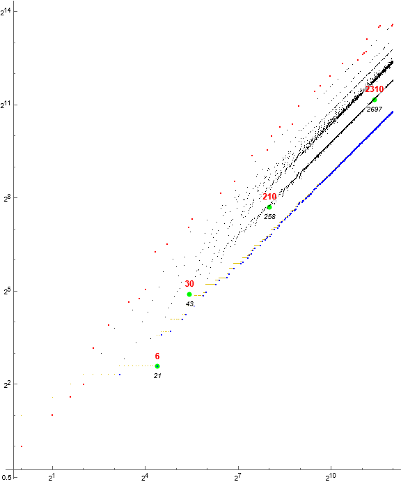
This effect detains strongly 3-smooth numbers but quickly abates as n increases and admits more p | s(n) : p > 3 into the sequence so as to furnish a greater range or vocabulary of distinct odd prime divisors of a and c to allow 6 | d to enter. The effect applies mildly to other primorials P(k) (numbers that occupy local minima for the ratio φ(n)/n) but likewise abates as k increases. Small multiples mP(k) suffer a similar delay that wears off as m increases.
Figure 2.1: Log-log scatterplot of s(n), 1 ≤ n ≤ 256, highlighting the trajectory of strongly 3-smooth numbers g in 6 R6 = 6 × A3586. These multiples of 6 are delayed early in the sequence.
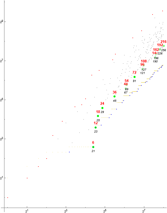
Figure 2.2: Log-log scatterplot of s(n), 1 ≤ n ≤ 212, highlighting the trajectory of primorials P in A2310. The effect of minimalized totient abates quickly.
General alignment of 2p with ℓ > 1 and introduction of prime p.
Odd run length ℓ = 3 associates with primes p = s(n) such that s(n−2) = 2p and s(n+2) = 4p.
Let P3 be the sequence of primes p associated with odd run length 3, that is, that have an odd term before and after p. This sequence begins:
17, 29, 37, 47, 61, 67, 71, 79, 89, 101, 103, 109, 131, 137, 157, 163, 173, 181, 199, 227, 241, 251, 269, 277, 281, 293, 311, 317, 347, 353, 359, 367, 379, 389, 401, 409, 419, 431, 443, 457, 463, 479, 487, 491, 499, 509, 523, 547, 569, 571, 587, 593, 599, 607, 617, 643, 647, 673, 677, 683, ...
Odd run length ℓ = 4 associates with primes p = s(n) such that s(n−2) = 2p and s(n+2) = 3p.
Let P4 be the sequence of primes p associated with odd run length 4, that is, that have an odd term before and after p followed by an additional odd term. This sequence begins:
7, 59, 149, 193, 211, 233, 263, 331, 373, 557, 563, 631, 659, 661, 727, 743, 823, 863, 971, 983, 1009, 1019, 1031, 1093, 1109, 1117, 1151, 1181, 1237, 1289, 1301, 1361, 1367, 1423, 1433, 1447, 1483, 1493, 1511, 1523, 1567, 1601, 1609, 1613, 1627, 1637, 1693, 1709, 1733, 1741, 1747, 1987, 2039, 2081, 2137, 2141, 2179, 2237, 2243, 2281, ...
Most primes associate with extended-run-length of odd terms. Those that do not must have mixed-parity neighbors:
2, 3, 5, 11, 13, 19, 23, 31, 41, 43, 53, 73, 83, 97, 107, 113, 127, 139, 151, 167, 179, 191, 197, 223, 229, 239, 257, 271, 283, 307, 313, 337, 349, 383, 397, 421, 433, 439, 449, 461, 467, 503, 521, 541, 577, 601, 613, 619, 641, 653, 691, 719, 733, 757, 797, 821, 827, 857, 907, 929, 937, 967, 997, 1051, 1063, 1091, 1097, 1123, 1187, 1217, 1231, 1291, 1303, 1327, 1427, 1439, 1453, 1471, 1481, 1487, 1571, 1607, 1619, 1723, 1759, 1873, 1931, 1951, 1979, 1999, 2029, 2143, 2153, 2239, 2293, 2309, 2389, 2411, 2549, 2593, 2659, 2689, 2699, 2741, 2803, 2963, 3019, 3041, 3301, 3313, 3323, 3389, 3677, 3881, 3923, 3931, 4079, 4139, 4243, 4271, 4289, 5021, 5113, 5869, ...
Even s(n) may satisfy (s(n−2), s(n)) > 1 often through s(n) ± 2, trine s(n) may satisfy (s(n−2), s(n)) > 1 via s(n) ± 3. Generally, if p = lpf(s(n)), then s(n) ± p are the closest values that satisfy (s(n−2), s(n)) > 1. Usually we find p | s(n) → s(n) + p i.e., kp → (k + 1)p since the smaller s(n) − p = (k − 1)p is more likely to already appear in s. If the factor p | kp is the first occasion of such in s, then we have kp → p, since p < kp has not already appeared in the sequence.
Consequently, even d arising from composite b appear in a central trajectory, while even d arising from prime b appear in a different trajectory. This is to say that primality of b bifurcates the magnitude of even d. Specifically, through observation, if we have prime b = s(n) and an even s(n+2), then we have d = 4b.
Figure 2.3: Log-log scatterplot of a(n) for 1 ≤ n ≤ 216, showing odd terms in blue and even in red. The upper red line is QLS α4, while the larger lower red line is QLS central γ-even.
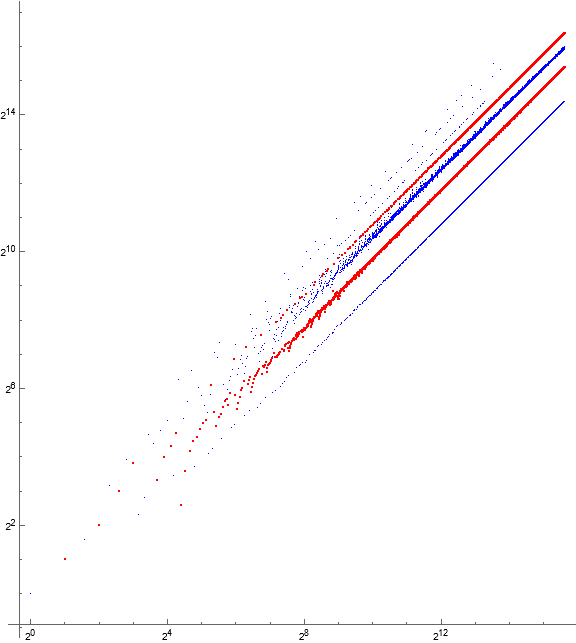
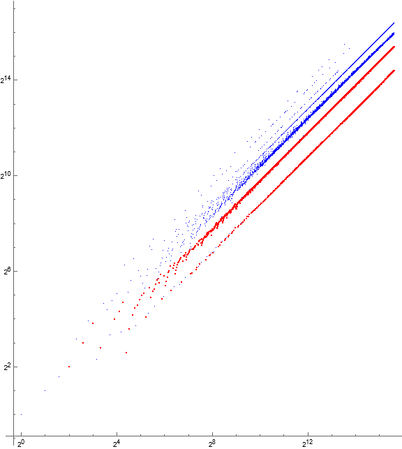
Figure 2.4: Log-log scatterplot of a(n) for 1 ≤ n ≤ 216, showing odd b in blue and even in red. This figure shows that primes p often generate even mp : m = 4, hence QLS α4. QLS central γ-even often generate other even terms in γ.
Primality.
Primes d are forced into divisibility since coprimality and equality are forbidden. Consequently, we have the following chain around prime terms p = s(n):
s(n−2) = kp > p < mp = s(n+2) : k ≠ m.
The effect of the prime-induced chain above is that s(n±2) differs from s(n) by multiples, necessitating a move away from the general trajectory of the sequence. In contrast, nearly all composite s(n) differ from s(n±2) by small addends and form a dense trajectory γ in s near slope 1:1. Therefore the appearance of primes p in s forces extremes.
Figure 3.1: Log-log scatterplot of a(n) for 1 ≤ n ≤ 216, showing composite terms in blue and prime in red. The primes occupy the trajectory of minima as a consequence of divisibility forced upon primes.
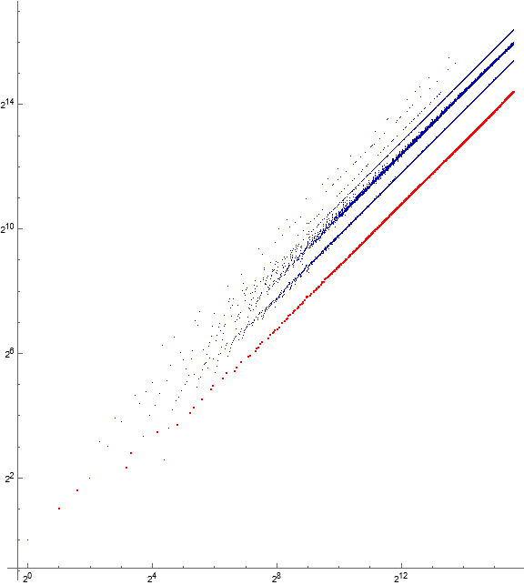
The primes occupy a trajectory β of minima, and s(n+2) : s(n) = p appear in a family of trajectories α with slopes greater than that of γ, since k < m except in three cases, s(26..30), s(46..50), and s(98..102). These are likely the only cases, since for n > 13679, apparently, k = 2 ∧ m > k.
For example, regarding s(100) = 43:
95, 96, 97, 98, 99, 100, 101, 102, 103, ...
(1) (1) (2) (4) (1) constitutive state of odd-indexed terms
82, 185, 84, 215, 88, 43, 92, 129, 94, ...
(1) (1) (1) (1) constitutive state of even-indexed terms
s(96) = 185 = 3³ × 5, therefore either 3 | s(98) or 5 | s(98). Since s(97) = 84 = 2² × 3 × 7, we must have the latter, hence we have the next multiple of 5 not in the sequence yet coprime to s(97), and this is 5 × 43. There is nothing to rule out another instance of k > m, except the minimization of k as n increases.
Consider the subsequence of consecutive terms that includes the prime p, i.e., {kp, x, p, y, mp}. Let us call this a “prime subsequence”.
Certainly, the “sandwiching” neighbors s(n−1) = x and s(n+1) = y are such that x ⊥ kp ∧ y ⊥ mp, therefore x and y are coprime to p, but k and m are free to have a common divisor or not. Introductory kp influences the parity of x, such that if 2 | kp, then x is odd, else potentially even. Generally, if (certainly extant) prime q | kp : q > p, then q ⊥ x and p follows x in the sequence. In a similar way, y influences the parity of m. If y is even, then m is odd, but odd y permits m of either parity.
We observe the Lagarias-Rains-Sloane chain in A064413:
2p → p → 3p
Under similar circumstances, and with 1 exception, kp introduces novel p into s; the appearance of p | kp is the largest prime factor seen in s for n > 4, otherwise p would have followed, representing a persistently smallest missing number. By same token, s(n+2) = mp : m ≠ k on account of the prohibition of coprimality and equality of a(n) and a(n+2).
The exception relates to s(19) = 26, which instead introduces a strongly delayed s(21) = 6 instead of 13.
Prime factors of the interposing term y and k influence m. The latter ensures m ≠ k, but the former affects parity and magnitude of m. Early k suffer influence from s(n−4) in that, if k is prime k | s(n−4) else (k, s(n−4)) > 1. Therefore unlike in the EKG sequence, we may have k > 2, and since new terms must always be the least available, k is indeed always prime. Indeed, if k ≠ 2, then k = 3 through influence of factors of s(n−4). It is possible that k might exceed 3, but this becomes less probable as n increases.
An effect of coprime neighbors is that, if k is even, often m is as well, hence k = 2 and m = 4, and if k is trine (i.e., 3 | k) and no trine terms appear between, we have trine m as well, hence k = 3 and m = 9. We may also see k = 3 and m in {5, 7} provided 6 | s(n+1) or s(n+1) 7- or 11-rough. There are only 10 possible k-m arrangements for prime p. Two of these pertain to given primes 2 and 3 (that is, m = 2 and m = 3 respectively). Then we have k in {2, 3, 5, 7} and m in {2, 3, 4, 5, 7, 9}.
Odd k implies odd m, since 2 | s(n ± 1). In contrast, if k = 2, then m = 3 iff s(n+1) mod 3 ≡ ±1, else m = 4, since s(n−1..n+1) are odd.
The usual mode in this sequence is k = 2, m = 4, a configuration that becomes more prominent as the sequence matures. Because k = 2 forces odd x and y normally resonates with parity of x, we are prone to m = 4. Of course, even y is not prohibited provided some other factor greater than 1 divides both x and y. If y is even (and it is more likely even than odd), then we have m = 3 instead. The case 6 | y would force m = 5 but never is seen to arise.
If k = 3, we may have m ∈ {5, 7, 9}. Generally, m ≤ k² per observation.
Primes may appear adjacently. Adjacent primes are found starting at the following indices:
2, 9, 501, 621, 1891, 1961, 2840, 3350, 3413, 3715, 4509, 5523, 6226, 9855, 9925
These are the 15 pairs of adjacent primes found in the dataset (see Table C):
{2, 3}, {5, 7}, {227, 229}, {269, 271}, {821, 823}, {853, 857}, {1229, 1231}, {1451, 1453}, {1481, 1483}, {1607, 1609}, {1949, 1951}, {2383, 2389}, {2687, 2689}, {4241, 4243}, {4271, 4273}
The prime subsequences associated with adjacent primes are intercalated. An example is s(7..12):
15, 14, 5, 7, 25, 21
There are no triples or longer runs of adjacent primes. Are there any more adjacent primes?
Table 3.1. Observed combinations km combined with parity of x and y in a dataset of 220 terms. Code 6 generates a table like this. Asterisked figures represent the number of terms in the dataset; these signatures are likely infinite in number, therefore there isn’t a last term.
mod 2 First Last
km xy card. n s(n) n s(n)
------------------------------------------------
2 11 1 2 2 2 2
3 00 1 3 3 3 3
23 11 10075* 10 7 1048590* 466787*
24 11 28773* 37 17 1048515* 466751*
35 00 49 62 31 9970 4289
35 01 5 9 5 9925 4271
35 10 9 502 229 9856 4243
37 00 40 18 11 13677 5869
39 00 16 171 73 11884 5113
53 00 1 100 43 100 43
73 00 1 48 23 48 23
75 00 1 28 13 28 13
The effect of the prime-induced chain therefore is to situate p in the trajectory of minima, β, followed by a term mp that appears in a trajectory αm.
We note that k = 2 associates with x and y both odd and k > 2 generally with x and y both even except in rare cases of k = 3 with mixed parity of x and y.
The k-m signature “23” is about a third as common as “24” and both associate with both x and y odd. This implies that y is nontrine so as to allow m = 3 in cases of signature “23”. Indeed, we find that both x and y are nontrine when m = 3 in all cases of “23”. The signature “24” has 3 divide at least 1 of x or y, if not both. Most commonly, 3 divides both x and y, and 3 | y is more common than 3 | x when k = 2 and m = 4. See Table A for a study akin to Table 3.1 but regarding x mod 3 and y mod 3.
The sequence A350359 does not mature until the k-m signatures outside those involving k = 2 go extinct for n > 13677. This implies that primes associate with odd x and y increasingly as n increases.
Why do the other k-m signatures go extinct? Is it true that these signatures are extinct? Why do large primes for n > 13677 associate with x and y both odd? These questions remain open.
Scatterplot features.
There are several major quasi-linear striations (QLS) in scatterplot. Let’s review from lowest to highest apparent slope. We realize that, since the recursive mappings of the function f do not use index n as input, we are not dealing with algebraic lines, but instead, with quasi-linear trajectories associated with general displacement between b and d that are strongly reliant on primality. For this reason we refer to the apparent rays or lines in the scatterplot as trajectories or QLS.
This recognition does not nullify the importance of slope analysis of s(n)/n, but instead is a different way of analyzing data. Aside from an aggregate apparent slope achieved by taking the mean of s(n)/n in a specific trajectory, the analysis of apparent slopes is beyond the scope of this work. Herein we use the term “slope” only in reference to apparent slope as described above.
Beta or minima trajectory.
Primes appear as local minima along with 1, 4, 6, and 12 as a consequence of definition of sequence forcing asymmetric divisibility. The primes in A350359 comprise the bottom-most QLS β in Figure 1. The mean slope of β ≈ 0.432244.
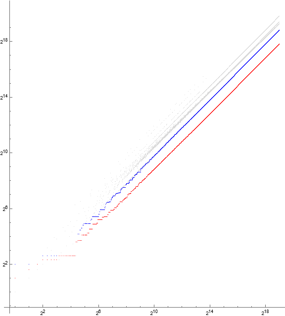
Composite numbers respect a composite local minima v instead of the absolute local minima u, aiding in computation. (See Code 1A)
Figure 4.1: Log-log scatterplot of s(n) for 1 ≤ n ≤ 219 superimposing the absolute local minima u consisting of primes and 1, 4, 6, and 12 in red, and the composite local minima v in blue.
Gamma or central trajectory.
Central γ QLS contains d ≠ mp mentioned in the prime section above such that both b and d are composite, bifurcated by parity. We define central γ as follows:
γ = s \ (αm ∪ β)
The constraint (b,d) > 2 bifurcates the central trajectory into an even and an odd stream, on account of the most common 2k → 2k ± 2, generally, qk → qk ± q, favoring upward moves except in the case of prime k. Thus, for q = 2, we most often have | b − d | = 2, for q = 3, we often have | b − d | = 3 (unless 2 | k, then it is possible to have | b − d | = 2), and generally | b − d | = q less frequently as q increases. Therefore we have a clearly even stream and a clearly odd stream that has more variation or “fuzz”, but in actuality the odd stream is a mix of odd moves dominated by moves of 3. Furthermore, the influence of sandwiching x and y terms before and after k tends to encourage coherent parity. If k is even, then y must be odd, and the term m that follows y may be either even or odd, but is likely even since (k + 2) is more likely available and (k + 1) ⊥ k. Given odd k, we may have even or odd y, but even y is more likely especially if x is also even. Therefore we have two streams of central trajectory:
Central γ-even, both b and d composite. Mean slope ≈ 0.863341.
Central γ-odd, both b and d composite. Mean slope ≈ 1.26518.
This implies that even terms tend to enter later than odd terms.
Alpha or prime-multiple trajectories.
Primes b force b | d thus b < d, therefore these cast terms in several fine and sparse QLS in the α zone.
There are 6 QLS defined by mp, where p is a prime s(n−2), and with m in {2, 3, 4, 5, 7, 9}.
α2 : d = 2b ∧ b prime, contains s(4) = 4 = 2 × 2. Slope d/n = 1.
α3 : d = 3b ∧ b prime, first term s(5) = 9 = 3 × 3. 1185 observed terms likely infinite. Falls within central γ-odd until it decouples around n = 48000, then lies at a generally higher apparent “slope”. Mean slope ≈1.29596. (See enlarged scatterplot for decoupling of α3 and γ-odd evident at extreme top right corner, the upper black fuzzy line that is splitting into a fuzzy line and a fine thread slightly above.)
α4 : d = 4b ∧ b prime, first term s(39) = 68 = 4 × 17. 3224 observed terms, likely infinite. Mean slope ≈1¾.
α5 : d = 5b ∧ b prime, first term s(11) = 25 = 5 × 5. 64 terms, largest is s(9970) = 4289, thereafter the trajectory is perhaps extinct. Mean slope ≈ 2.16909.
α7 : d = 7b ∧ b prime, first term s(20) = 77 = 7 × 11. 40 terms, largest is s(13679) = 41083, thereafter the trajectory is perhaps extinct. Mean slope ≈3.07224.
α9 : d = 9b ∧ b prime, first term s(173) = 657 = 9 × 73. 16 terms, largest is s(11886) = 46017, thereafter the trajectory is perhaps extinct. Mean slope ≈3.88969.
Figure 4.2: Log-log scatterplot of a(n) for 1 ≤ n ≤ 214, color coded to show αm for m = 2 (gold), m = 3 (red, within central γ-odd), m = 4 (orange), m = 5 (blue), m = 7 (green), m = 9 (magenta).
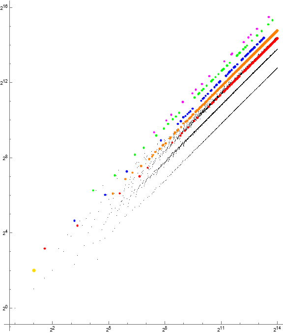
Many records r occur in QLS αm. Records r have ω(r) = 2 in most cases, but 2, 3, 4, 9, 25, and 27 appear early. QLS α4 conspicuously sets records beginning with s(26813) = 46076, since it appears that αm for m > 4 have been exhausted.
Generate a list of indices of terms in αm with Code 3.
Figure 4.3: Log-log scatterplot of s(n) for 1 ≤ n ≤ 216 showing maxima r in red and minima t in blue. The golden line indicates the least unused number u. The α4 records at upper right indicate that αm : m > 4 have stopped appearing for n > 13679. What is the reason? (Code 8 generates this scatterplot. See an enlarged scatterplot of s(n) for 1 ≤ n ≤ 218.)
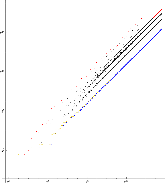
Conjecture: there are 5 infinite trajectories: α4, α3, γ-odd, γ-even, and β.
Trajectory β contains primes p by definition, in order of their magnitude and serving as local minima as a consequence of generally prohibited equality and prohibited coprimality of b and d, forcing primes p into divisibility.
Trajectory α3 has prime b and composite d, and both x and y are both odd and nontrine when m = 3. Therefore s(n−3) and s(n−1) belong to 1 or 5 (mod 6), s(n−2) is prime p, and s(n) = 3p for terms in trajectory α3.
Trajectory α4 has prime p = b and composite d. The factor 3 divides at least 1 of x or y, if not both, and both x and y are necessarily odd, for prime p and m = 4. Therefore s(n−3) and s(n−1) are odd but 3 divides at least 1 of these, while s(n−2) is prime p, s(n−4) = 2p and a(n) = 4p for terms in trajectory α4.
Trajectories α4 and γ-even contain even terms; those in γ-even relate to b and d both composite.
Trajectory γ contains composite terms that are not preceded by a(n−2) prime. The trajectory is bifurcated into an early odd γ-odd, and a later γ-even stream as a consequence qk → qk ± q, favoring upward moves except in the case of prime k. Thus, for q = 2, we most often have | b − d | = 2, for q = 3, we often have | b − d | = 3 (unless 2 | k, then it is possible to have | b − d | = 2), and generally | b − d | = q less frequently as q increases.
Powers 2ε : ε < 1 appear in γ-even, while pε : ε > 1 ∧prime p > 2 appear in γ-odd.
The superposition of α3 and γ-odd is not yet explained. The trajectories are independent and “decouple” in the interval 215 < n < 216. QLS γ-odd arises from composite b while α3 is produced by prime b, hence the answer lies in the differences between the general trajectory of composites (in γ) and primes (in β). We surmise that QLS α3 and QLS γ-odd further spread apart as n increases. (See enlarged scatterplot for decoupling of α3 and γ-odd evident at extreme top right corner, the upper black fuzzy line that is splitting into a fuzzy line and a fine thread slightly above.)
Interference of prime systems connected with extinction of αm : m > 4.
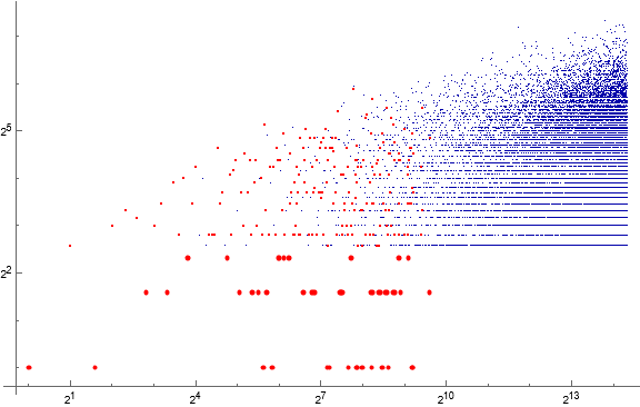
The apparent extinction of trajectories αm : m > 4 seems to have to do with the early chance availability of k > 2 and parity of x and y. It may have to do with the interference of prime subsequences when they are intercalated or sufficiently adjacent. This stands to reason given the degree of agitation caused by primes in s, and the reverberation of parity in every other term.
Figure 4.4: Log-log scatterplot of first differences D of primes. Highlighted D ≤ 5 seem conspicuously confined under a certain threshold. The last term highlighted in red (D = 3 and n = 772) pertains to s(13674) = 5867 and s(13677) = 5869.
Constitutive Analysis.
See this paper on constitutive analysis, which relates to numbers d in the cototient of b and vice versa.
Table 5.1 summarizes the constitutive binary relations and their qualities. Examples appear in the note. For coprimality, we may consider any 2 dissimilar primes p and q. Symmetrical divisibility applies only to j = k, which is forbidden.
| C | | | binary relation | abb. | sym. | neut. | reg. | rev. | note |
| ---- | | | ------------------ | ------ | ------ | ------ | ------ | ------ | ---------------- |
| ⓪ | | | j ⊥ k ∧ k ⊥ j | ⊥ | ✓ | ⓪ | ∀ p, q, p ≠ q | ||
| ① | | | j ◊ k ∧ k ◊ j | ◊.◊ | ✓ | ✓ | ① | 6, 10 | |
| ② | | | j ◊ k ∧ k | j | ◊.| | ④ | 30, 6 | |||
| ③ | | | j ◊ k ∧ k || j | ◊.|| | ✓ | ⑦ | 30, 12 | ||
| ④ | | | j | k ∧ k ◊ j | |.◊ | ② | 10, 30 | |||
| ⑤ | | | j | k ∧ k | j | |.| | ✓ | ✓ | ⑤ | ∴j = k | |
| ⑥ | | | j | k ∧ k || j | |.|| | ✓ | ⑧ | 6, 12 | ||
| ⑦ | | | j || k ∧ k ◊| j | ||.◊ | ✓ | ③ | 20, 30 | ||
| ⑧ | | | j || k ∧ k | j | ||.| | ✓ | ⑥ | 20, 10 | ||
| ⑨ | | | j || k ∧ k || j | ||.|| | ✓ | ✓ | ✓ | ⑨ | 12, 18 |
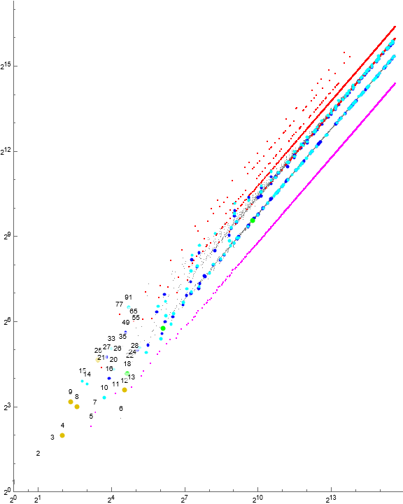
Most common state is completely neutral, symmetrically semicoprime ① that requires b and d both composite. The next most commonly seen states are ② and its reverse, ④ (pertains to primes) then by ③ and its reverse, ⑦ (pertains to prime powers not prime). Because all the primes appear and the sequence is infinite, there are infinite numbers of states ①②③④⑦ in s.
We see a usually even term kp transform via state ② to yield an odd prime p which is the greatest prime factor of kp. Its reverse transforms p via state ④ into mp, with m often even. In other words, p | kp, and p | mp, but kp and mp each have a factor distinct from one another and from p (i.e., k and m respectively) that does not divide prime p by definition of prime.
State ⑥ represents a collision effect between primes and prime powers not prime: 2 ⑥ 4, 3 ⑥ 9, 4 ⑥ 8, 5 ⑥ 25, 6 ⑥ 12. These are the only instances of state ⑥ in the sequence. State ⑥ occurs between adjacent prime powers pε : ε ≥ 0, where the former power is smaller than the latter, but also between certain members of the sequence RK, that is, terms that are products limited to the factors of squarefree kernel K. Its reversal is state ⑧. These states are rare on account of the sparsity of RK.
State ⑧ is absent but may be ruled out by similar reasons to Bob Selcoe’s observation in A098550. It likely does not exist since it occurs between numbers j and k : k | j therefore j > k, that have the same squarefree kernel K, e.g., 12 ⑧ 6, K = 6, both are 3-smooth numbers in A3586 = R6. Due to the sparsity of numbers in RK, if the state were to appear in the sequence, it would have appeared early.
State ⑨ appears at s(23) = 12 ⑨ 18, s(67) = 48 ⑨ 54, and s(881) = 720 ⑨ 750. It should prove ever rarer as n increases. This state did not appear in the EKG sequence and only appears here on account of the agitation produced by sandwiching terms x and y.
We have one seed instance of 1 ⓪ 3, that is, 1 coprime to 3, which is forbidden, but occurs on account of the definition of the sequence.
Powers 2ε : ε > 1 appear in γ-even, while pε : ε > 1 appear in γ-odd. We see states ② introducing terms in βand ④ terms in α. The neutral states ①③⑦⑨ appear in γ. State ⑥ is a defect of state ④. We expect ⑧ to appear in γ-even.
Generate a sequence of constitutive states between terms using Code 4.
Constitutive signatures.
Constitutive signatures include ②_④ and ③_⑦, pertaining to primes and prime powers not prime, respectively, as similar signatures do in A064413. Furthermore, there are intercalations of these signatures and collisions that are either trivial or easily explained in the first couple dozen terms in the sequence. See Table D for a list of intercalations and collisions of ②_④, and Table E for same pertaining to ③_⑦.
There are no isolated cases of states ② or ④, that is, outside of association with prime subsequences however defective. These require a divisor relationship and the only possible such relationships are when n is small and unless s(n) is prime. This is a consequence of selecting the least unused d and the other constraints.
There are singleton or isolated cases of states ③, ⑦, and ⑨, which are defects of state ①. These cases exchange semicoprimality for assymetric or symmetric semidivisibility. The case s(881) = 720 ⑨ 750 is the sole isolated case of state ⑨.
Isolated state ③ occurs at the following indices n:
194, 224, 774, 1021, 1165, 1445, 1508, 2251, 3746, 5661, 5788, 5938, 6007, 9300, 9601, 12075, 14181, 14623, 15118, 16478, 21487, 23301, 29781, 36322, 37190, 41802, 57856, 60514, 60709, 70142, 71788, 84947, 107712, 114828, 117535, 128996, 135363, 160082, 168648, 192733, 200472, 340573, 445739, 452859, 454434, 531986, 592685, 594191, 730240, 738516, 747670, 806420, 844075, 902989, 948595, 1035283, ...
Isolated state ⑦ occurs at the following indices n:
256, 468, 1606, 1695, 1788, 2098, 2693, 3195, 3390, 4017, 7013, 11933, 23651, 27214, 27981, 28622, 29084, 40087, 62495, 63932, 86415, 119055, 178599, 182842, 224188, 224472, 267744, 270301, 291112, 314218, 353011, 371682, 398056, 401616, 445241, 475203, 489856, 500366, 529955, 533960, 562254, 624168, ...
It is curious that we have not seen isolated state ⑦ for over 400000 terms after the last-listed appearance.
Conjecture: there are infinite numbers of singleton states ③ and ⑦, since the constraint (b, d) > 1 does not restrict b-regular d or vice-versa, despite the rarity of pairs of numbers b and d as these increase in magnitude. In contrast, there are no more cases of state ⑨, since it requires b ∈ RK ∧ d ∈ RK : (K = rad(b) ∧ rad(d)), where RK is a sparse infinite sequence akin to a geometric progression.
Table 5.2: Summary of constitutive states in A350359 given a dataset of 220 terms. Asterisked states are infinite in number: ② and ④ associate with primes, ③ and ⑦ with prime powers not prime, and ① transpires amid composites. Generate this table using Code 4 and Code 5:
Even Prime
State n b d card. b d b d
-------------------------------------------------------------
(0) 1 1 3 1 - - - 1
(1) 17 20 26 969895 441302 451366 - -
(2) 7 15 5 38969 38847 - - 38969
(3) 12 21 27 373 131 131 - -
(4) 10 7 21 38968 - 28773 38968 -
(5) ----- forbidden equality -----
(6) 2 2 4 5 3 3 3 -
(7) 5 9 15 362 118 128 - -
(8) --- unlikely unless small ----
(9) 23 12 18 3 3 3 - -
Signature catenation, intercalation, and collision.
In the EKG, Yellowstone, and Olson’s sequence, the prime ②④ and prime power ③⑦ signatures in those sequences at times occur consecutively, catenating states outside of state ①. In this sequence, because of the structure of constraints, the prime and prime power signatures can intercalate as well as append.
For instance, we may have consecutive primes and thus have an intercalated signature ②②④④, or we may have primes separated by 2 nonprime terms so as to have a catenated signature ②_④②_④. This also applies to prime powers not prime so as to have ③③⑦⑦ or ③_⑦③_⑦, respectively, though the latter is not observed and probably never arises.
We may also have mixed intercalated states or mixed conjoined states, thus, ②③④⑦ or ③②⑦④, or ②_④③_⑦ or ③_⑦②_④ respectively.
We may have isolated state ③ or ⑦ appended to the above signatures. We even have 2 cases of straddled isolated states, i.e., ②③④ but ②⑦④ has not been seen. The state ⑥ represents the collision of prime p and prime powers pε : ε > 1 ∧ p | pε, separated by 1 term coprime to both (i.e., indivisible by p).
We have ②_④ → __⑥_⑥ in the case of 2 → 4 → 8, and ②_④ → ⓪_⑥ in the case of (1 →) 3 → 9; these are intercalated so as to obtain ⑥⑥⑥ at the start of a conglomeration of 15 states exclusive of ①. The first prime resulting from directive, 5, corrupts ②_④ → ②_⑥, via 15 → 5 → 25 → 10 intercalated with the subsequence associated with 7 to obtain ②②⑥④⑦. There is a pair of consecutive prime powers {27, 16} that appends ③③⑦⑦ to the conglomeration. The subsequence of 11 appears at the end of the conglomeration, appending ②①④.
Table 5.3 lists the conglomerated signatures seen in a dataset of 220 terms.
Signature card. n s(n)
---------------------------------------------------------------------------
32_4 2 1470 1270,1923,1280,641
2_42_4 23 37 17,57,68,19
2_43 2 1025 886,1445,443,1365,1772
2_43_7 27 178 79,231,316,243
2_47 7 38 57,68,19,40,133,30
72_4 1 111282 137781,96926,137823,48463
234 2 218 190,291,182,97,196,485
2244 13 499 454,687,227,229,908,1145
2347 19 449 386,575,193,529,579,460
3274 19 56 75,58,81,29,93,116
3377 4 70 115,62,125,64,105,74
6397 1 21 6,35,12,49,18,91
32742_4 1 56 75,58,81,29,93,116,31
33773_7 1 149 247,126,169,128,221,132,289
3_72347 2 17819 22201,15286,22499,7643,22801,22929,15704
666772264733772 1 2 2,3,4,9,8,15,14,5,7,25,21,10,27,16,33,20,11
Figure 5.3: Log-log scatterplot of a(n) for 1 ≤ n ≤ 216, color-coded to show constitutive states between b and d. Tiny gray dots have state ①, medium-sized dark blue ③, medium-sized cyan ⑦, comprising central γ. Magenta dots correspond to p and state ② in QLS β. Red dots correspond to 3p and state ④ in QLS αm. Large gold dots pertain to state ⑥. State ⑨ appears in green.
Prime powers not prime.
Prime powers appear in order such that pε precedes p(ε+1), however, prime powers generally are not arranged in order seen in A1694.
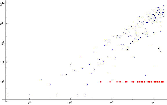
An interesting situation arises in the sequence regarding certain consecutive prime squares s(n) = p² and s(n+4) = q². The phenomenon is conspicuous in the scatterplot of first differences of indices n of prime powers not prime in A350359 shown by Figure 5.4.
Table 5.3: Occasions of prime squares that appear 4 terms apart in A350359, with the first prime at s(n), in a dataset of 220 terms.
p^2 q^2
n s(n) s(n+4) q-p
------------------------------
522 29^2 31^2 2
1481 43^2 47^2 4
2864 59^2 61^2 2
4120 71^2 73^2 2
8169 101^2 103^2 2
9226 107^2 109^2 2
15049 137^2 139^2 2
17819 149^2 151^2 2
25693 179^2 181^2 2
31181 197^2 199^2 2
41523 227^2 229^2 2
46105 239^2 241^2 2
58536 269^2 271^2 2
79043 313^2 317^2 4
88686 331^2 337^2 6
98071 347^2 349^2 2
116754 379^2 383^2 4
152315 431^2 433^2 2
174607 461^2 463^2 2
204218 499^2 503^2 4
223864 521^2 523^2 2
267647 569^2 571^2 2
315514 617^2 619^2 2
340861 641^2 643^2 2
360545 659^2 661^2 2
491853 769^2 773^2 4
546597 809^2 811^2 2
563199 821^2 823^2 2
571496 827^2 829^2 2
614274 857^2 859^2 2
614278 859^2 863^2 4
649670 881^2 883^2 2
872679 1019^2 1021^2 2
893736 1031^2 1033^2 2
925482 1049^2 1051^2 2
947076 1061^2 1063^2 2
1002094 1091^2 1093^2 2
Figure 5.4: Log-log scatterplot of first differences D of indices of prime powers not prime in A350359. The plot highlights occasions of D = 4, which are distances between certain consecutive prime squares.
Conclusion.
The “sandwich sequence” exhibits sociable behavior sensitive to primality and parity of adjacent and nearby terms. It is comparable to the EKG, Yellowstone, and Olson (A347113) sequences that restrict terms j and k to ( j, k) > 2. These sequences exhibit a sorting process that casts primes into minima on account of prohibited coprimality and equality; they are relegated to divisorship of neighboring terms. Therefore, these sequences feature an introductory predecessor kp and a resultant mp that exhibit jumps in the sequence, whereas composite terms generally vary much less between neighbors. The sequences feature quasi-linear striations that are trajectories that tend to respond to parity and primality as a consequence of the definitions of the sequences.
OEIS A350359 differs from the other sequences in the requirement of two alternating streams of terms, odd-indexed and even-indexed, that have terms that are coprime to adjacent terms. This “sandwiching” distorts the relationship patterns most purely conveyed by the EKG sequence. The adjacent coprimality requirement enhances the effect of parity in this sequence.
Like the EKG sequence, there is a somewhat clear progression associated with primes akin to the Lagarias-Rains-Sloane chain. Constitutive signatures are likewise similar to those in EKG.
The question of “maturation” of the sequence concerns the extinction of trajectories or quasi-linear striations (QLS) αm : m > 4. Perhaps this occurs at n = 13679, because s(13679) is the last term of α7 trajectory. It might instead be seen as n = 26813, since all records after s(26813) concern terms in α4. We may perhaps instead consider A350359 “mature” only upon the clear decoupling of trajectories α3 and γ-odd after n > 48000. It seems that about 217-218 terms of A350359 clearly exhibit all expected behavior of the sequence.
The extinction of the trajectories αm : m > 4, entailing that both s(n−1) and s(n+1) are odd for prime s(n) : n > 13679, remains an open question. What has changed in the sequence after so many terms that prohibits even neighbors of primes?
See Table A for landmark terms in the sequence.
This concludes our examination.
Appendix.
Table A. General landmarks in A350359.
Constitutive states explained at the constitutive census and the constitutive signature segment of this work. See Table C for a list of 15 pairs of adjacent primes in the sequence.
s(1..3) = {1 ⓪ 2 ⓪ 3}; given terms.
s(2..3) = {2, 3}; smallest known pair of adjacent primes.
s(2) = 2, only prime with m = 2, i.e., s(4) = 2 × 2 = 4. First instance of rare state ⑥: 2 ⑥ 4.
s(3) = 3, first prime with m = 3, i.e., s(5) = 3 × 3 = 9; 3 ⑥ 9.
s(4) = 4 = mp for m = 2, p = 2; only term in α2 “trajectory”; 4 ⑥ 8.
s(5) = 9 ⑦ 15 = s(7); first instance of state ⑦.
s(7) = 15 ② 5 = s(9); first instance of state ②.
s(9) = 5; first instance of k-m pattern “35”, first such with even x, odd y; 5 ⑥ 25.
s(10) = 7; first instance of apparently infinite k-m pattern “23”. First instance of state ④: 7 ④ 21.
s(12) = 21 ③ 27 = s(14); first instance of state ③.
s(17) = 20 ① 26 = s(19); first instance of the most common state ①.
s(18) = 11; first instance of k-m pattern “37”.
s(19) = 26; only instance of kp that introduces a composite rather than p.
s(21) = 6; last instance of rare state ⑥: 6 ⑥ 12. Strongly detained term on account of slight totient.
s(23) = 12; first instance of rare state ⑨: 12 ⑨ 18.
s(26) = 91 = 7 × 13, s(30) = 65 = 5 × 13; Only instance of k-m pattern “75”.
s(13) = 13, Only instance of a prime p that did not follow the first kp in the sequence.
s(46) = 161 = 7 × 23, s(50) = 69 = 3 × 23; Only instance of k-m pattern “73”.
s(62) = 31; first instance of k-m pattern “35” with even x = 116, even y = 56.
s(67) = 48 ⑨ 54.
s(98) = 215 = 5 × 43, s(102) = 129 = 3 × 43; Only instance of k-m pattern “53”.
s(171) = 73; first instance of k-m pattern “39”.
s(194..195) = 156 ③ 162; first instance of isolated state ③.
s(256..257) = 216 ③ 210; first instance of isolated state ⑦.
s(502) = 229; first instance of k-m pattern “35” with odd x = 227, even y = 908.
s(881) = 720 ⑨ 750, last instance of rare state ⑨, a strong singleton state, last instance of nonstandard states (not ①②③④⑦). Constitutive maturation of the sequence.
s(9148) = 3929, s(9153) = 3931; largest prime pair spaced 5 terms apart in s.
s(9856) = 4243; last instance of k-m pattern “35” with odd x = 4243, even y = 16964.
s(9925..9926) = {4271, 4273}; largest (known) pair of adjacent primes.
s(9925) = 4271; last instance of k-m pattern “35” with even x = 8546, odd y = 4273.
s(9970) = 4289, last prime with m = 5; largest instance of k-m pattern “35” (with x and y both even).
s(9972) = 21445 = 5 × 4289, last term of α5 trajectory.
s(11884) = 5113, last prime with m = 9; largest instance of k-m pattern “39”.
s(11885) = 46017 = 9 × 5113, last term of α9 trajectory, last record set by αm : m > 4.
s(13674) = 5867, s(13677) = 5869; largest prime pair spaced less than 6 terms apart in s.
s(13677) = 5869, last prime with m = 7; largest instance of k-m pattern “37”.
s(13679) = 41083 = 7 × 5869, last term of α7 trajectory.
s(26813) = 46076 = 4 × 11519, first record in α4 trajectory after extinction of αm : m > 4.
(Constitutive state ⑧ has not yet appeared given 218 terms, which though not prohibited, likely does not exist since it occurs between numbers j and k that have the same squarefree kernel K.)
Table B. Observed combinations km combined with x mod 3 and y mod 3 for a dataset of 220 terms.
The table shows that k = 2 ∧ 3 | x ∧ 3 | y ∧ m = 4 is the most common arrangement for primes in A350359. Return to Table 3.1 akin to this table, but instead regarding parity. Asterisked figures pertain to the dataset; the signatures are likely infinite in number and there are no last terms.
mod 3 First Last
km xy card. n s(n) n s(n)
-------------------------------------------------
2 10 1 2 2 2 2
3 22 1 3 3 3 3
23 11 967* 751 331 1048590* 466787*
23 12 4094* 135 59 1048299* 466651*
23 21 4036* 10 7 1047863* 466451*
23 22 978* 537 233 1048571* 466777*
24 00 14940* 37 17 1048515* 466751*
24 01 2350* 501 227 1047561* 466321*
24 02 2461* 1564 673 1048093* 466561*
24 10 4585* 234 101 1048350* 466673*
24 20 4437* 158 67 1048436* 466717*
35 11 6 1154 503 7058 3041
35 12 16 412 179 9153 3931
35 21 18 9 5 9970 4289
35 22 23 62 31 9856 4243
37 11 3 342 151 4064 1759
37 12 14 84 41 7710 3323
37 21 14 40 19 11683 5021
37 22 9 18 11 13677 5869
39 11 4 797 349 7664 3301
39 12 3 494 223 5579 2411
39 21 7 321 139 11884 5113
39 22 2 171 73 269 113
53 12 1 100 43 100 43
73 22 1 48 23 48 23
75 10 1 28 13 28 13
Table C. Complete list of adjacent prime pairs or duplex primes.
i n s(n) s(n+1) n+1
------------------------------------
1 s(2) 2 3 s(3)
2 s(9) 5 7 s(10)
3 s(501) 227 229 s(502)
4 s(621) 269 271 s(622)
5 s(1891) 821 823 s(1892)
6 s(1961) 853 857 s(1962)
7 s(2840) 1229 1231 s(2841)
8 s(3350) 1451 1453 s(3351)
9 s(3413) 1481 1483 s(3414)
10 s(3715) 1607 1609 s(3716)
11 s(4509) 1949 1951 s(4510)
12 s(5523) 2383 2389 s(5524)
13 s(6226) 2687 2689 s(6227)
14 s(9855) 4241 4243 s(9856)
15 s(9925) 4271 4273 s(9926)
Table D. List of signatures ②_④ that pertain to primes, showing first instance at s(n), and the number of instances seen in the dataset of 220 terms. The number of ②①④ signatures is infinite.
sig. n s(n) card.
-----------------------
214 18 11 38900*
224 501 227 13 (complete signature 2244)
226 9 5 1 (complete signature 2264)
234 221 97 21 (complete signature usually 2347)
244 502 229 13 (complete signature 2244)
264 10 7 1 (complete signature 2264)
274 59 29 19 (complete signature 3274)
Table E. Complete list and ③_⑦.
sig. n s(n) card.
-----------------------
317 72 125 207*
327 73 64 19 (complete signature 3274)
337 24 49 3 (complete signature 3377)
347 522 841 19 (complete signature 2347)
377 33 32 4 (complete signature usually 3377)
397 58 81 1
647 15 16 1
666 6 8 1
667 11 25 1
677 14 27 1
Code 1: Efficiently generate s and store it in the variable a350359.
a350359 = Block[{s = Range[3], a, b, c, k, u = 1, r}, r[_] = 0;
Array[Set[r[s[[#]]], #] &, Length[s]];
Set[{a, b, c}, s[[-3 ;; -1]]]; While[r[u] > 0, u++];
s~Join~Reap[Monitor[Do[If[c == u, While[r[u] > 0, u++]]; k = u;
While[Nand[r[k] == 0, CoprimeQ[a, k], CoprimeQ[c, k], GCD[b, k] > 1], k++];
Sow[k]; r[k] = i; a = b; b = c; c = k, {i, Length@ s + 1, 2^12}], i]][[-1, -1]]]
Code 1A: Efficiently extend s and store it in the variable a350359, taking advantage of the composite local minimum.
a350359 = Block[{s = a350359, a, b, c, k, u = 1, w = 1, r},
r[_] = 0;
Array[Set[r[s[[#]]], #] &, Length[s]];
Set[{a, b, c}, s[[-3 ;; -1]]];
If[r[12] > 0, While[r[u] > 0, u = NextPrime[u]],
While[r[u] > 0, u++]]; While[Nand[r[w] == 0, ! PrimeQ[w]], w++];
s~Join~Reap[Monitor[Do[
If[c == u,
If[r[12] == 0, While[r[u] > 0, u++],
While[r[u] > 0, u = NextPrime[u]]]];
If[c == w, While[Nand[r[w] == 0, ! PrimeQ[w]], w++]];
If[r[12] == 0, k = u;
While[Nand[r[k] == 0, CoprimeQ[a, k], CoprimeQ[c, k], GCD[b, k] > 1], k++],
Which[
Mod[b, u] == 0, k = u,
PrimeQ[b], k = 2;
While[Nand[r[b k] == 0, CoprimeQ[a, b k], CoprimeQ[c, b k]], k++]; k = b k,
True, k = w;
While[Nand[r[k] == 0, CoprimeQ[a, k], CoprimeQ[c, k], GCD[b, k] > 1], k++]]];
Sow[k]; r[k] = i; a = b; b = c; c = k, {i, Length@ s + 1, 2^16}], i]][[-1, -1]] ]
Code 2: Generate auxiliary sequences d(n) = τ(a(n)), u(n) = least unused number, r = maxima, s = local minima, indices of primes (pi) and prime powers not prime (ppi), and parity (pp).
a350359d = Map[GCD[#1, #3] & @@ # &, Partition[a350359, 3, 1]];
a350359u = Block[{u = 1, c, s = a350359}, c[_] = 0;
Reap[Do[Set[c[s[[i]]], i]; If[s[[i]] == u, While[c[u] > 0, u++]];
Sow[u], {i, Length@ s}]][[-1, -1]]];
a350359r = Union@ FoldList[Max, a350359];
a350359s = Union@ a350359u;
a350359pi = Position[a350359, _?PrimeQ][[All, 1]];
a350359ppi = Position[a350359, _?(And[PrimePowerQ[#], ! PrimeQ[#]] &)][[All, 1]];
a350359pp = Mod[a350359, 2];
Code 3: Generate indices n pertaining to αm and store in dimensioned variable alpha[m], and the sequence a350359pr of multipliers m : mp = s(n+2) for prime s(n) = p.
a350359pr = Map[Divide @@ a350359[[{# + 2, #}]] &, a350359pi];
Table[Set[alpha[k],
Select[Range[3, Length[a350359]],
And[PrimeQ[a350359[[# - 2]]], a350359[[#]]/a350359[[# - 2]] == k] &]],
{k, Union[a350359pr]}];
Code 4: Generate constitutive states between terms:
a350359c = With[{s = Partition[a350359, 3, 1]},
Function[{a, b}, {0}~Join~(1 +
Rest@ Array[3*(1 + a[[#]]) + (1 + b[[#]]) &,
Length[a]])] @@
{Map[
Which[Mod[#3, #1] == 0, 0,
PowerMod[#3, #3, #1] == 0, 1,
True, -1] & @@ # &, s],
Map[
Which[Mod[#1, #3] == 0, 0,
PowerMod[#1, #1, #3] == 0, 1,
True, -1] & @@ # &, s]}];
Code 5: Generate constitutive census Table 5.2:
Block[{nn = 2^10, s, t, j = 2},
s = a350359[[1 ;; nn + 2]];
t = a350359c[[1 ;; nn]];
Map[{
StringJoin["(", ToString[#1], ")"], #2, #3, #4, Count[t, #1],
With[{k = #1}, Count[Position[t, k][[All, 1]], _?(EvenQ@ s[[#]] &)]],
With[{k = #1}, Count[Position[t, k][[All, 1]], _?(EvenQ@ s[[# + j]] &)]],
With[{k = #1}, Count[Position[t, k][[All, 1]], _?(PrimeQ@ s[[#]] &)]],
With[{k = #1}, Count[Position[t, k][[All, 1]], _?(PrimeQ@ s[[# + j]] &)]]} & @@
Flatten@ {#1, #2, s[[#2]], s[[#2 + 2]]} & @@
{#, FirstPosition[t, #][[1]]} &, Union@ t]] // TableForm
Code 6: Generate an assessment of k-m classes with parity shown such that suffix 0 = both even, 1 = m odd, k even, 2 = m even, k odd, and 3 = both even. Similar to Table 3.1:
a350359ppp = {2, 3}~Join~
Map[FromDigits[{Divide[#1, #3], Divide[#5, #3],
FromDigits[{Mod[#2, 2], Mod[#4, 2]}, 2]}] & @@
a350359[[# - 2 ;; # + 2]] &, a350359pi[[3 ;; -1]]];
With[{t = Union@ a350359ppp},
Map[{#1, #2, #3, a350359[[#3]], #4, a350359[[#4]]} & @@
{#1, #2, a350359pi[[#3]], a350359pi[[#4]]} & @@
Flatten@ {#, Count[a350359ppp, #],
Position[a350359ppp, #][[{1, -1}, 1]]} &, t]] // TableForm
(The case k mod 3 and m mod 3 is easily derived from above).
Code 7: Generate Figure 1.1:
Block[{nn = 2^6, a, r, s, u, out = -120},
a = a350359[[1 ;; nn]];
r = Array[If[FreeQ[a350359r, #], out, #] &@ a[[#]] &, nn];
s = Array[If[FreeQ[a350359s, #], out, #] &@ a[[#]] &, nn];
u = a350359u[[1 ;; nn]];
ListPlot[{a, a, s, r, u,
Array[Labeled[#, #, Top] &@ a[[#]] &, nn],
Array[If[FreeQ[a350359r, #], out,
Labeled[#, #, Top, LabelStyle -> Red]] &@ a[[#]] &, nn],
Array[If[FreeQ[a350359s, #], out,
Labeled[#, #, Bottom, LabelStyle -> Blue]] &@ a[[#]] &, nn]
},
ImageSize -> Large,
ScalingFunctions -> {"Log2", "Log2"},
AspectRatio -> Automatic,
Joined -> {True, False, False, False, False, False},
PlotStyle -> {Directive[Gray, Thin],
Directive[Black, PointSize[Medium]],
Directive[Blue, PointSize[Large]],
Directive[Red, PointSize[Large]],
Directive[Hue[1/7, 1, .875], PointSize[Tiny]],
Transparent, Transparent, Transparent
} ]]
Code 8: Generate Figure 4.3:
Block[{nn = 2^16, a, r, s, u, out = -120},
a = a350359[[1 ;; nn]];
r = Array[If[FreeQ[a350359r, #], out, #] &@ a[[#]] &, nn];
s = Array[If[FreeQ[a350359s, #], out, #] &@ a[[#]] &, nn];
u = a350359u[[1 ;; nn]];
ListPlot[{a, u, s, r},
ImageSize -> 1920,
ScalingFunctions -> {"Log2", "Log2"},
AspectRatio -> Automatic,
PlotStyle -> {
Directive[Black, PointSize[Tiny]],
Directive[Hue[1/7, 1, .875], PointSize[Tiny]],
Directive[Blue, PointSize[Small]],
Directive[Red, PointSize[Small]]
} ]]
Concerns sequences:
A064413: the EKG sequence.
A098550: the Yellowstone sequence.
A347113: Olson’s sequence.
Document Revision Record.
2021 1228 1345 Final.
2021 1228 2300 Observations of prime and prime power spacing.
2021 1229 0930 Update for 219 term dataset.
2021 1230 0930 Update regarding 6, 13, and s(19)
2021 1231 0800
Update for 220 term dataset.
2021 1231 1900 Update for catenated constitutive signatures.