On a recursive coprimality sequence.
Written by Michael Thomas De Vlieger, St. Louis, Missouri, 2020 1118.
Abstract.
We examine three recursive self-referential integer sequences that deal with the coprimality of a novel nonzero positive k with either the last term, the partial sum of the sequence hitherto, or both, starting with the first term 1. The concept for this paper derives from David Sycamore.
In this work we use the term “trine” to signify a number k ≡ 0 (mod 3), i.e., divisible by 3, while “nontrine” signifies a number k indivisible by 3.
Introduction.
We may write a sequence z, setting z(1) = 1, thereafter, z(n + 1) is the least novel nonzero positive k that is coprime to z(n). Since 2 is the least prime and therefore we cannot find a prime divisor common to n and n ± 1 (ignoring n < 1 in the case of n = 1), we see that z is tantamount to the sequence of natural numbers.
Consider OEIS A084385, that is, the sequence b(n) with b(1) = 1, thereafter, b(n + 1) is the least novel nonzero positive k that is coprime to the partial sum S = b(1…n). This sequence is a permutation of the natural numbers that begins:
1, 2, 4, 3, 7, 5, 9, 6, 8, 11, 13, 10, 12, 15, 17, 14, 16, 19, 21, 18, 20, 23, 25, 22, 24, 27, 29, 26, 28, 31, ...
b(2) = 2 since 2 is coprime to the partial sum 1.
b(3) = 4 since 3 | 3, but 4 is coprime to the partial sum 3.
b(4) = 3 since 3 is coprime to S = 7.
b(5) = 7 since, regarding S = 10, 5 | 10, gcd(6, 10) = 2, but gcd(7, 10) = 1.
b(6) = 5 since S = 17 is prime and 5 is the least unused number and happens to be a prime distinct from 7.
b(7) = 9 since 8 and 22 are even, but 9 is coprime to 22.
For n > 6:
b(n) = n − 2 for (n mod 4) = 0,
b(n) = n − 1 for (n mod 4) = 1,
b(n) = n + 1 for (n mod 4) = 2,
b(n) = n + 2 for (n mod 4) = 3.
We observe that for n > 6, the sum S cycles through the residues {1, 1, 0, 1, 2, 2, 3, 2} according to n mod 8.
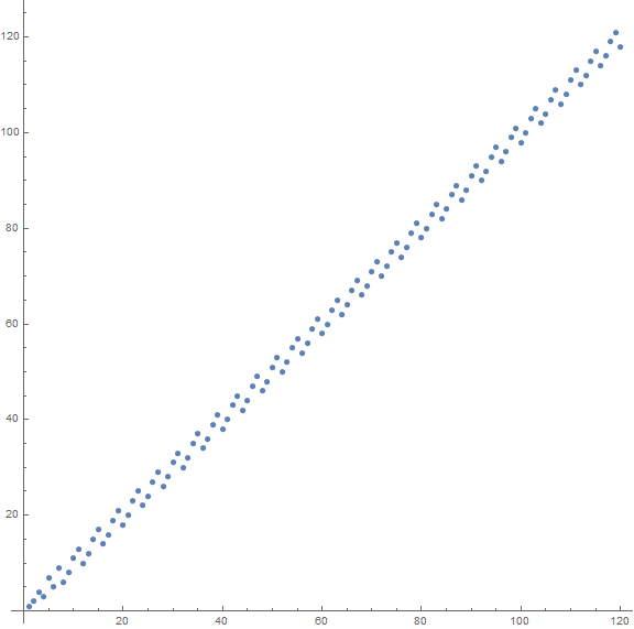
Figure 1.1 is a plot that demonstrates the regularity of the sequence b(n).
We now consider a sequence by Sycamore, a(n), whose partial sum is s(n), with a(1) = 1 and a(n + 1) the least k not already in the sequence such that gcd(k, a(n)) = gcd(k, s(n)) = 1.
The sequence begins:
1, 2, 5, 3, 4, 7, 9, 8, 11, 13, 10, 17, 19, 6, 29, 23, 12, 25, 31, 14, 37, 15, 16, 21, 41, 18, 35, 43, 22, 27, ...
a(2) = 2 since gcd(2, 1) = 1. (a(1) = 1 and s(1) = 1).
a(3) = 5 since a(2) = 2 and s(2) = 3, and 5 is the least number not already in a(n) that is coprime to both 2 and 3.
a(4) = 3 since a(3) = 5 and s(3) = 8, and 3 is the least unused number that is coprime to both 5 and 8.
a(5) = 4 since 4, the least unused number, is pairwise coprime to a(4) = 3 and s(4) = 11, etc.
The Plot of a(n).
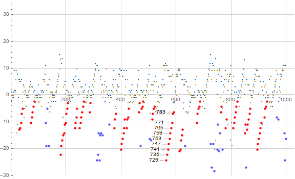
Figure 2.1 is a plot of a(n) for 1 ≤ n ≤ 1000, showing bifurcation into distinct “rays” that appear to be arranged about lines struck from the origin of slope 4/3 (blue) and 2/3 (red):
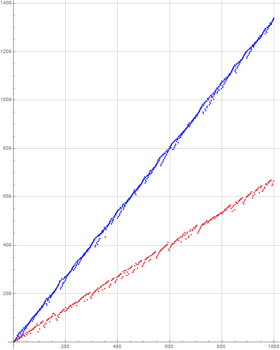
The upper ray shown in blue, with apparent slope of 4/3 contains odd values of a(n) while the lower ray shown in red, with apparent slope of 2/3 contains a(n) even. Both rays feature “leading fringe” terms that creep upward to a more solid yet irregular “barrier” of points. Generally, though the data associated with the rays exhibit turbulence, they do not vary much from the lines implied by their arrangements. There are twice as many terms in the upper ray than in the lower.
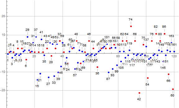
Figure 2.2 is a plot of a(n) for 1 ≤ n ≤ 120, labeling some of the points with (x, y) = (n, a(n)).
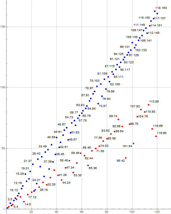
We note an additional correlation between rays and the index n. For n ≡ 2 (mod 3), a(n) is even and appear in the lower ray, otherwise a(n) is odd and appear in the upper ray.
Figure 2.3 plots a(n) for 1 ≤ n ≤ 240, labeling some of the points with (x, y) = (n, a(n)). We show the upper ray, dashing in a dark blue line from origin with slope 4/3, and the lower ray with a dark red dashed line from origin with slope 2/3. We indicate a(n) = r (mod 6), showing residue 0 in black and 3 in gray, 1 in brown and 4 in gold, 2 in blue and 5 in dark blue, so as to have odd residues appear grayed out.
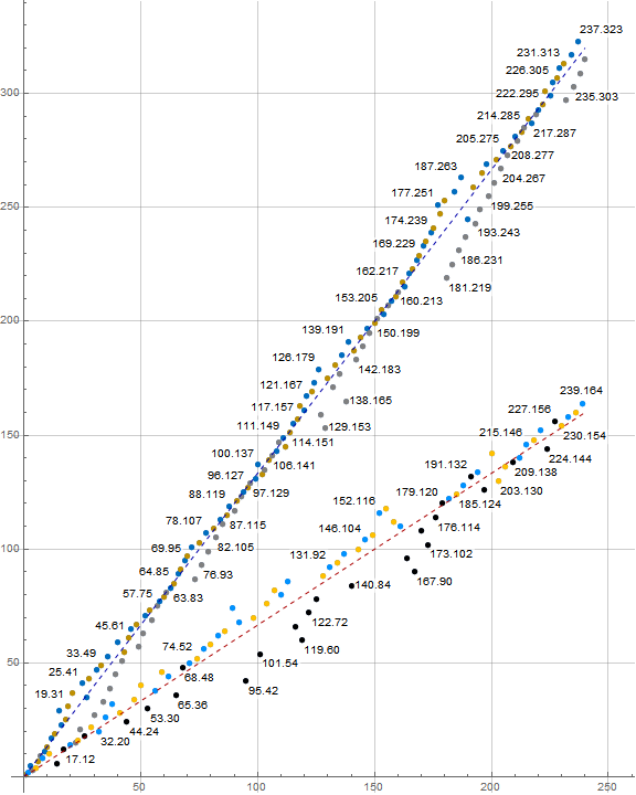
This figure demonstrates several things regarding a(n). Firstly, we see confirmed that odd a(n) appear in the upper line and thus enter a(n) “early” while even a(n) appear in the lower line and appear “tardy”. Furthermore, a(n) divisible by 3 appear relatively late with regard to the rays. This corroborates with the definition of the sequence, vis-a-vis pairwise coprimality with the partial sum and previous term. We do not observe any clear correlation between the congruence of n mod 6 and a(n) mod 6.
Examining the parity of a(n), there is a pattern that has a(n) even for n ≡ 2 (mod 3), else odd:
1, 2, 5, 3, 4, 7, 9, 8, 11, 13, 10, 17, 19, 11, 29, 23, …
This leads to the partial sum s(n) even for 3 | n:
1, 3, 8, 11, 15, 22, 31, 39, 50, 63, 73, 90, 109, 115, 144, 167, 179, 204, 235, 249, 286, …
There doesn’t seem to be a pattern in the residues of s(n) mod 6, except that 6 | s(n) is rare, and s(n) mod 6 ≡ ±1 is common, the former to the latter in an approximate 1:4 ratio.
Likewise, we find the occasion of relatively long runs of even a(n) such that a(n) mod 6 ≡ 0; within n < 100000, there is a run of 9 such even a(n). In Figure 3 there is evident a run of 4 even a(n) mod 6 ≡ 0 (shown in black) for n in {116, 119, 122, 125}, and of 6 even a(n) immediately following the interposing singleton.
The association of the upper ray with a slope of 4/3 and the lower ray with 2/3 enables us to “undercut” the data by setting the iterator to fall 100 units below the rays and efficiently generate the sequence. The sequence was generated from k = 2 for 1 ≤ n ≤ 5000, but we generated 10000 terms using the undercutting method.
Examination of the congruence bifurcation.
Earlybirds and laggards in each ray.
We now turn to the nature of the two rays, the upper ray (blue) with slope m = 4/3 and the lower (red) with slope m = 2/3. In these congruence-related streams, we can identify numbers that occur “early”, and further, numbers that are extreme “earlybirds”, as well as those that appear “late”, and further, numbers that are extreme “laggards” with relation to the streams. We know that the upper ray contains odd a(n) while the lower ray contains even a(n), which stands to reason given the definition of a(n). Thus, we may as well see the upper ray as itself an early ray, and the lower ray as a late ray. Here we are trying to determine what is the nature of numbers a(n) that appear ahead of “schedule” (i.e., above the line of slope m) and those that appear behind “schedule” (i.e., below the line of slope m). For the upper and lower rays, numbers a(n) divisible by 3 have a strong tendency to appear behind schedule, while those indivisible by 3 have a mild tendency to appear a bit ahead of schedule.
We now turn our attention to earlybirds that set records for earliness, and laggards that set records for tardiness in both rays. The following data is gleaned from a dataset of a(n) with 1 ≤ n ≤ 100 000.
Figure 3.1 is a plot of a(n) − mn showing 1 ≤ n ≤ 1200 for n belonging to 0 or 1 (mod 3). We indicate the earlybirds with large red and the laggards with large blue dots:
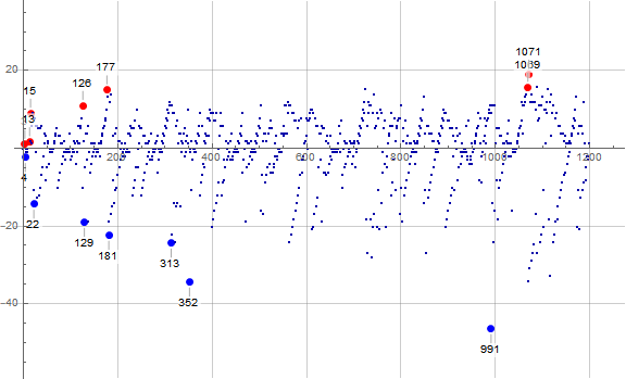
Earlybirds in the upper (blue) ray of slope m = 4/3, with d = 3(a(n) − mn):
i n a(n) d
-----------------------
1 3 5 3
2 13 19 5
3 15 29 27
4 126 179 33
5 177 251 45
6 1069 1441 47
7 1071 1447 57
8 2371 3181 59
9 10693 14279 65
10 13209 17635 69
11 23142 30881 75
These a(n) tend to be odd primes, though 1441, 14279, and 17635 are odd squarefree semiprimes 11 × 131, 109 × 131, and 5 × 3527, respectively.
Laggards in the upper (blue) ray of slope m = 4/3, with d = 3(mn − a(n)):
i n a(n) d
-----------------------
1 4 3 7
2 22 15 43
3 129 153 57
4 181 219 67
5 313 393 73
6 352 435 103
7 991 1275 139
8 3402 4485 153
9 19210 25545 205
Aside from a(n) = 3, these laggards are odd composites, with generally increasing numbers of distinct prime divisors.
Figure 3.2 is a plot of a(n) − mn showing 1 ≤ n ≤ 1200 for n ≡ 2 (mod 3). We indicate the earlybirds with large red and the laggards with large blue dots:
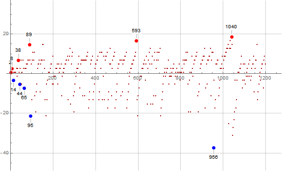
Earlybirds in the lower (red) ray of slope m = 2/3, with d = 3(a(n) − mn):
i n a(n) d
----------------------
1 2 2 2
2 8 8 8
3 38 32 20
4 89 74 44
5 593 412 50
6 1040 712 56
7 14897 9952 62
8 19265 12866 68
This list contains some a(n) that are perfect powers of 2 as well as even composites with relatively few factors compared to the even laggards.
Laggards in the lower (red) ray of slope m = 2/3, with d = 3(mn − a(n)):
i n a(n) d
-----------------------
1 14 6 10
2 44 24 16
3 65 36 22
4 95 42 64
5 956 600 112
6 14930 9912 124
7 30035 19980 130
8 30311 20160 142
9 39146 26040 172
This list contains even and trine a(n) (that is, a(n) ≡ 0 (mod 6)) that have relatively many factors compared to the earlybirds, however we do not see all highly divisible a(n) here.
Earlybirds and laggards mod 6.
Figure 3.3 is a plot of a(n) − mn showing 1 ≤ n ≤ 1200 for n belonging to 0 or 1 (mod 3), which has a(n) odd. This plot shows a(n) ≡ 1 (mod 6) in brown, a(n) ≡ 3 (mod 6) in gray, and a(n) ≡ 5 (mod 6) in dark blue. Most of the odd earlybirds and laggards are called out and shown with a large dot:
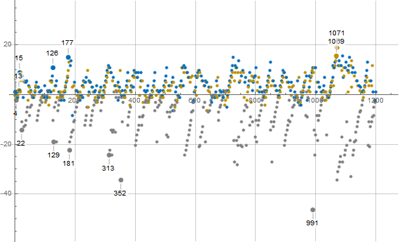
It is plain to see that we have odd earlybirds belonging to both 1 and 5 (mod 6) but the odd laggards are congruent to 3 (mod 6), at least in this domain. We conjecture that the odd laggards are always congruent to 3 (mod 6). Additionally, we generally see that a(n) ≡ 5 (mod 6) generally come into the sequence earlier than a(n) belonging to any other residue (mod 6).
Click here for an enlarged plot of this odd (blue) ray in the style of Figure 3.3 showing 1 ≤ n ≤ 215. The enlarged plot seems to support the notion that the departure from a line from origin of slope m = 4/3 is reflected in “iceberg” fashion above and below the line. When we have a(n) ≡ 3 (mod 6) in black excessively low on the graph, we see a(n) with the other odd residues (mod 6) above the line, their departures less prominent.
Each of these odd residues (mod 6) might be examined for their own earlybirds and laggards. (See Appendix).
Figure 3.4 is a plot of a(n) − mn showing 1 ≤ n ≤ 1200 for n ≡ 2 (mod 3), which generates even a(n). This plot shows a(n) ≡ 0 (mod 6) in black, a(n) ≡ 2 (mod 6) in blue, and a(n) ≡ 4 (mod 6) in gold. Most of the odd earlybirds and laggards are called out and shown with a large dot:
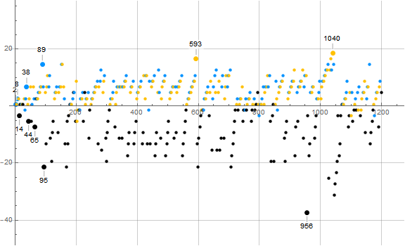
We can see that we have even earlybirds belonging to both 2 and 4 (mod 6) but the even laggards are congruent to 3 (mod 6), among the data shown. We conjecture that the even laggards are always congruent to 0 (mod 6), that is, even and trine. Additionally, we generally see that a(n) ≡ 2 (mod 6) generally come into the sequence earlier than a(n) belonging to the other even residues (mod 6).
Click here for an enlarged plot of this even (red) ray in the character of Figure 3.4 showing 1 ≤ n ≤ 215. The enlarged plot seems to support the notion that the departure from a line from origin of slope m = 2/3 is reflected in “iceberg” fashion above and below the line. When we have a(n) ≡ 0 (mod 6) in black excessively low on the graph, we see a(n) with other even residues (mod 6) above the line, their departures less prominent. Compared to the enlarged plot of the odd ray, we see that the even ray indeed is half as dense as the odd, which stands to reason given the parity of n and the residues of a(n) (mod 3) that result.
Overlay of the rectified plots of bifurcations.
We examine the upper (odd, early, blue) and lower (even, late, red) rays, specifically, the apparent “ladder” like structures that are same-parity a(n) increasing as n increases. These structures appear in the rectified plots along the requisite slopes m, but we know that in actuality, there are terms that interpose of opposite parity. How do the two streams interrelate? Do we see ladders in the odd stream (upper ray) accompanied by anything in the even (lower ray)?
Figure 3.5 collapses even and odd a(n) via plotting a(n) − (2 + 2 (a(n) mod 2))/3. Many of the points are labeled with the value of a(n) rather than the plotted function. (View a plot for 1 ≤ n ≤ 3600)
Here we see that there doesn’t seem to be a correlation between the points. However it stands to reason that even k, appended to a(n), do not alter the parity of S while odd k do. Therefore, as to parity, the even a(n) prove inconsequential.
Examination of the congruences of a(n + 1), a(n), and s(n), mod 6.
We find that, in contrast to the cyclical behavior of b(n) mod 4, that a(n) experiences a particular behavior mod 6.
If either a(n) or s(n) is even, or both are even, k must be odd. Thus, the only time k may be even is in the case where both a(n) and s(n) are odd. Similarly, k may be trine only when both a(n) and s(n) are nontrine. Generally, we have p | k only when p divides neither a(n) nor s(n). Because of this, we have a chaotic assortment of a(n) mod 6, yet we see that a(n) ≡ 2 (mod k) for n even.
k = 2 is even following odd a(1) = 1 and s(1) = 1.
k = 5 is odd given even a(2) = 2 and odd s(2) = 3.
k = 3 is odd given odd a(3) = 5 and even s(3) = 8, and we see the influence of parity of k on s(n).
k = 4 is even given odd a(4) = 3 and odd s(4) = 11.
k = 7 is odd given even a(5) = 4 and odd s(5) = 15.
k = 9 is odd given odd a(6) = 7 and even s(6) = 22.
k = 8 is odd given odd a(7) = 9 and even s(7) = 31. We see k = 6 detained, and the development of a reservoir of small even numbers.
Generally, only one of k, a(n), and s(n) may be even. Since the sequence a(n) starts with 1 and s(n) the partial sum of 1, both odd, we are allowed an even k for n ≡ 2 (mod 3) *. This changes the parity of a(n) but not s(n), and prevents even k, therefore the parities of a(n) and s(n) swap, again preventing even k. The entrance of odd k for n ≡ 1 (mod 3) flips the parity of s(n) but retains an odd a(n), setting the stage for the next even k for n ≡ 2 (mod 3). This situation repeats ad infinitum for n > 21. Hence the association with the lower ray with both n ≡ 2 (mod 3) and even a(n), with odd n and a(n) belonging to 0 or 1 (mod 3) in the upper ray. There are twice as many a(n) in the upper ray as in the lower for this reason. The slopes are 4/3 and 2/3 since there is a parity effect that rotates every 3 n, and the least unused number k is relatively never far from entering the sequence.
* The least unused k is always even for n > 21, but before this, the least unused k is odd only on 4 occasions, none of which are when n ≡ 2 (mod 3).
Congruence mod p for prime p ≥ 5.
It seems that the sequence is governed by parity and divisibility mod 3 mainly on account of the truth table that admits an even k only for a(n) and s(n) both odd, coupled with the rotation of parity amid the three variables. The seeming order mod 6 is really only sensitive to parity and divisibility by 3. This seems to be a reason why we do not see a meaningful sensibility mod 5 or any larger prime p, except that 6p | k tend to be found latest, 3p | k late compared to other odd k, especially when p is small.
The “ladder” phenomenon.
We see a series of “sticky” k — relatively highly divisible terms — enter the sequence late, followed by a string of consecutive terms that are congruent to 3 (mod 6). The sticky, least term k in the ladder is sometimes a multiple of a perfect power of an odd prime, normally 3. Until this sticky k enters the sequence, many of the others in the ladder cannot enter since they share some of the same divisibility properties as the sticky k. This is merely an observation; a rigorous analysis hasn’t been performed.
Similar effects are observed for the even (lower, red) ray.
Laggards and highly composite k.
The sorting of trine a(n) in the tardy sides of the line with slope m in either ray is an effect of dodging divisibility by 3 or any other prime so as to furnish a k coprime to both a(n) and s(n).
Are there occasions of extremely delayed k? These k would be even and trine and likely relatively highly divisible, but it is difficult to predict exactly which k.
Primorials are not highly composite outside of 2 and 6, yet we can find these at indices n ≡ 2 (mod 3):
n a(n) d
-------------------
2 2 2
14 6 -10
53 30 -16
326 210 -22
3500 2310 -70
45089 30030 -88
Again, d = 3(a(n) − 2n/3). Therefore, positive values appear early (i.e., a(n) < 2n/3) and negative late as expected.
The highly composite numbers (A2182) appear as follows:
n a(n) d M(a(n))
------------------------------
1 1 1 0
2 2* 2 1
5 4 2 2
14 6* -10 11
17 12 2 21
44 24* -16 31
65 36* -22 22
68 48 8 41
119 60 -58 211
179 120 2 311
299 180 -58 221
374 240 -28 411
554 360 -28 321
1091 720 -22 421
1289 840 -58 3111
1922 1260 -64 2211
2555 1680 -70 4111
3797 2520 -34 3211
7574 5040 -28 4211
11357 7560 -34 3311
15128 10080 -16 5211
22715 15120 -70 4311
30311 20160* -142 6211
37832 25200 -64 4221
41612 27720 -64 32111
68048 45360 -16 4411
75638 50400 -76 5221
83171 55440 -22 42111
The column M(a(n)) contains the exponents of the prime divisors p | a(n), written in the π(p)-th place.
Of these highly composite k, only 2, 6, 24, 36, and 20160 are (even) absolute laggards, meaning that they set records for tardiness overall.
Issues for further exploration:
1. Does the sequence a(n) exist? We perhaps have not made a full case based on congruences that the patterns shown here hold.
This concludes our examination of this sequence; more may be added later.
Appendix:
Statistics on earlybirds and laggards for each residue mod 6, beginning with the odd (pertaining to the upper ray) and followed by even (lower ray).
Upper (odd, blue) Ray, slope m = 4/3.
a(n) ≡ 1 (mod 6)
Earlybirds Laggards
n a(n) d n a(n) d
------------------ ----------------
13 19 5 6 7 3
19 31 17 43 55 7
21 37 27 102 133 9
178 247 29 112 145 13
180 253 39 243 319 15
1066 1435 41 640 847 19
1069 1441 47 1243 1645 37
1071 1447 57 9277 12355 43
2371 3181 59 14005 18655 55
13209 17635 69 28182 37555 63
62244 83017 75
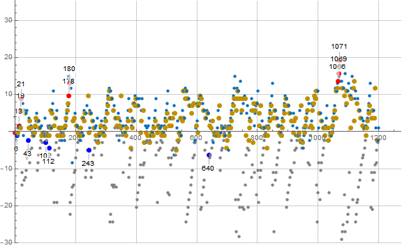
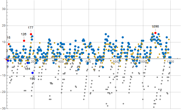
Figure A1: plot of a(n) − mn with m = 4/3 showing 1 ≤ n ≤ 1200 for n ≡ 1 (mod 6), highlighting earlybirds in red and laggards in blue:
a(n) ≡ 3 (mod 6)
Earlybirds Laggards
n a(n) d n a(n) d
------------------ -----------------
7 9 -1 4 3 7
109 147 5 22 15 43
2334 3117 15 129 153 57
12175 16239 17 181 219 67
21894 29199 21 313 393 73
352 435 103
991 1275 139
3402 4485 153
19210 25545 205
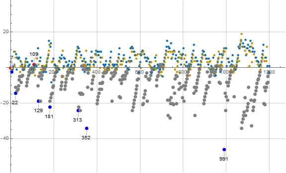
Figure A3: plot of a(n) − mn with m = 4/3 showing 1 ≤ n ≤ 1200 for n ≡ 3 (mod 6), highlighting earlybirds in red and laggards in blue:
a(n) ≡ 5 (mod 6)
Earlybirds Laggards
n a(n) d n a(n) d
------------------ ----------------
3 5 3 9 11 3
15 29 27 154 203 7
126 179 33 190 245 25
177 251 45 2397 3185 33
1090 1469 47 11604 15455 51
2821 3779 53 69718 92939 55
4539 6071 57
10693 14279 65
23142 30881 75
Figure A5: plot of a(n) − mn with m = 4/3 showing 1 ≤ n ≤ 1200 for n ≡ 5 (mod 6), highlighting earlybirds in red and laggards in blue:
Lower (even, red) Ray, slope m = 2/3.
a(n) ≡ 0 (mod 6)
Earlybirds Laggards
n a(n) d n a(n) d
------------------ ----------------
13 19 5 6 7 3
19 31 17 43 55 7
21 37 27 102 133 9
178 247 29 112 145 13
180 253 39 243 319 15
1066 1435 41 640 847 19
1069 1441 47 1243 1645 37
1071 1447 57 9277 12355 43
2371 3181 59 14005 18655 55
13209 17635 69 28182 37555 63
62244 83017 75
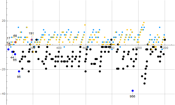
Figure A0: plot of a(n) − mn with m = 4/3 showing 1 ≤ n ≤ 1200 for n ≡ 0 (mod 6), highlighting earlybirds in red and laggards in blue:
a(n) ≡ 2 (mod 6)
Earlybirds Laggards
n a(n) d n a(n) d
------------------ -----------------
4 3 -7 4 3 7
7 9 -1 22 15 43
109 147 5 129 153 57
2334 3117 15 181 219 67
12175 16239 17 313 393 73
21894 29199 21 352 435 103
991 1275 139
3402 4485 153
19210 25545 205
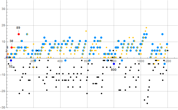
Figure A2: plot of a(n) − mn with m = 4/3 showing 1 ≤ n ≤ 1200 for n ≡ 2 (mod 6), highlighting earlybirds in red and laggards in blue:
a(n) ≡ 4 (mod 6)
Earlybirds Laggards
n a(n) d n a(n) d
------------------ ----------------
3 5 3 3 5 -3
15 29 27 9 11 3
126 179 33 154 203 7
177 251 45 190 245 25
1090 1469 47 2397 3185 33
2821 3779 53 11604 15455 51
4539 6071 57 69718 92939 55
10693 14279 65
23142 30881 75
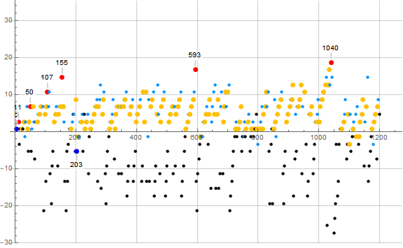
Figure A4: plot of a(n) − mn with m = 4/3 showing 1 ≤ n ≤ 1200 for n ≡ 4 (mod 6), highlighting earlybirds in red and laggards in blue:
Block[{a = {1}, s = 1, k},
Do[k = 2;
While[Nand[FreeQ[a, k], GCD[k, s] == 1], k++];
AppendTo[a, k]; s += k, 120]; a]
Block[{a = {1}, s = 1, k},
Do[k = 2;
While[Nand[FreeQ[a, k], GCD[k, a[[-1]] ] == 1, GCD[k, s] == 1], k++];
AppendTo[a, k]; s += k, 120]; a]
Code 3: Storing a(n) in variable a, generate Figure 2.3:
Block[{nn = 240},
Show[{ListPlot[
Array[Style[
Labeled[#2,
StringJoin @@ Riffle[Map[ToString, {#1, #2}], "."]],
Switch[Mod[#2, 6], 1, Hue[1/8, 1, .75], 2, Hue[4/7], 3, Gray,
4, Hue[1/8], 5, Hue[4/7, 1, .75], _, Black] ] & @@
{#, a[[#]]} &, nn],
ImageSize -> Large, AspectRatio -> Full,
GridLines -> Automatic] },
Graphics[{Thin, Dashed, Darker[Blue], Line[{{0, 0}, {nn, 4 nn/3}}],
Darker[Red], Line[{{0, 0}, {nn, 2 nn/3}}]}] ] ]]
Concerns OEIS sequences:
A084385 a(1) = 1; a(n+1) = least novel k coprime to the partial sum of a(n).
Document Revision Record.
2020 1118 2100 Created.
2020 1119 0745 Added earlybird and laggard observations.
2020 1119 1615 Added congruence remarks.