The Lazy Racer Sequence
A 2018 sequence by Rémy Sigrist, independently posed by David J. Sycamore in late 2020.
written by Michael De Vlieger 20 December 2020.
Abstract.
We examine behavior of a self-referential digit cardinality function, including cardinality trajectories in the original decimal (A322182). The sequence is regarded with Christmas humor of a “road race” where each trajectory is a “numbered car”. Do the cars “pass” one another? What is the nature of a “challenge on the race track”? What is the effect of “pole position”? What does a race between “more cars” look like? Therefore we regard the binary, ternary, senary, and sexagesimal version of the sequence as well.
Introduction.
Let s(1) = 1, s(n+1) is the number of times the nth digit in the sequence has been seen, up to and including itself. The sequence appears in OEIS at A322182.[1]
Therefore, given sequence s, we can write a second, auxiliary sequence t such that t(n) is the nth digit in s. We may define a counting function c(d,n) that registers the number of digits d in t(1..n). In this way, perhaps to facilitate writing an algorithm, we might define s(1) = 1, s(n+1) = c(d,n). It is clear that c(d,n) increments for each appearance of d in t, therefore c(d,n) strictly increases as n increases; when it increases it increases precisely by 1.
The sequence s begins:
1, 1, 2, 1, 3, 1, 4, 1, 5, 1, 6, 1, 7, 1, 8, 1, 9, 1, 10, 11, 1, 12, 13, 14, 15, 2, 16, 2, 17, 2, 18, 2, 3, 19, 2, 4, 20, 2, 5, 21, 2, 6, 3, 22, 2, 7, 3, 8, 2, 9, 3, 10, 23, 11, 3, 4, 12, 13, 14, 3, 5, 3, 15, 3, 6, 24, 3, 16, 7, 25, 26, 8, 4, 27, 17, 28, 9, 29, 5, 10, 4, 11, 30, 5, 12, 4, 18, 6, 13, 31, 5, 4, 19, 6, 20, 6, 4, 7, 21, 5, 32, 6, 22, 5, 4, 23, 5, 7, 33, 4, 8, 34, 35, 14, 5, 8, 36, 24, 9, 37, …
s(2) = 1 since t(1) = 1, and there has only been a single 1 in s thus far, so we write 1.
s(3) = 2 since t(2) = 1; there have been 2 digits 1 in s thus far.
s(4) = 1 since t(3) = 2, and we see only a single 2 in s so far.
...
s(18) = 1 since t(17) = 9, we’ve seen a single 9 thus far.
s(19) = 10 since t(18) = 1, and hitherto we have seen 10 digits 1.
s(20) = 11 since t(19) = 1; we have seen 11 digits 1 at this point.
(We note here that t(19) ≠ s(19), and hereafter, t is decoupled and distinct from s).
s(21) = 1 since t(20) = 0, the last number never before seen in s.
s(22) = 12 since t(21) = 12, since we’ve seen a dozen 1s thus far.
etc.
The algorithm that generates the sequence generates more terms than the number of iterations, since we are not referring to the previous term s(n − 1) to furnish s(n) for n > 19, but instead the (n − 1)-th digit in s. For the purposes of this essay, we have run 217 = 131072 iterations that yield 544297 terms of s(n), which equate to 2610421 digits.
Figure 1 is a plot of s(n) for 1 ≤ n ≤ 1000:
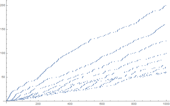
The plot shows 10 streams that represent c(d, n) for 0 ≤ d ≤ 9 that appear in t(1..n). Therefore the sequence s “autoanalyzes” itself, reporting the number of 1s, 2s, etc. that appear digit by digit in the sequence. We can use a color function related to the progenitor digit d = t(n) in order to distinguish the streams visually.
Figure 2 is a plot of s(n) for 1 ≤ n ≤ 120, with many points labeled s(n), and a color function rendering the progenitor digit d = t(n). Red indicates d = 1, orange d = 2, yellow d = 3, yellow green d = 4, green d = 5, cyan d = 6, blue d = 7, dark blue d = 8, magenta d = 9, and black d = 0. This link leads to an annotated and color-coded enlarged plot of 300 terms.
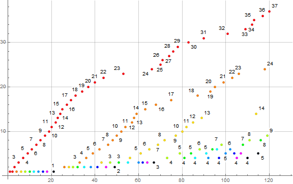
Figure 2 shows that each counting function c(d, n) increments by 1 upon each appearance of d in sequence s as it should.
We shall employ the same color function throughout for consistency.
The lazy racers.
We can think of the sequence s as a “race”. These streams can be thought of as race cars numbered d, with d = 1 in pole position, rocketing off at the start. d = 2 fires off, followed by the other digits in rough order, with d = 0 in last place.
Since there are 10 decimal digits, there are 10 race cars, never more, and for all values m in s, there are precisely 10 copies of m except for m = 1, for which there are 11, since we start with s(1) = 1.
Perhaps stating the obvious, for each n, precisely 1 racer advances by 1; when this racer advances, no other racers advance. As a consequence, the records transform of s is the sequence of the natural numbers (OEIS A27). We can efface the record-setters 9 times and the resultant new records remain the sequence of natural numbers, even if there is a pass, since the records in s are tantamount to an assay of the maximum number of times any one digit d appears in s(1..n).
Figure 3 is a plot of s(n) for 1 ≤ n ≤ 240, with many points labeled d for the digit d = t(n) → s(n+1).
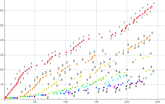
Figure 3 merely clarifies the notion of the racers or streams pertaining to progenitor digits d that are the n-th digit in the sequence s that result in the term s(n+1) = c(d, n), the number of digits d instantiated at the n-th digit in s (as opposed to the n-th term in s, which may and usually does regard a multiple-digit decimal number, outside of the first several dozen terms).
Figure 4 is a color-coded plot of s(n) for 1 ≤ n ≤ 214. Since we know there are 10 copies of m for m > 1, we indicate a dashed line with slope 1/10 on the graph. (Click this link for an extended and enlarged plot of 105 terms, or this link for a log-log plot of 105 terms):
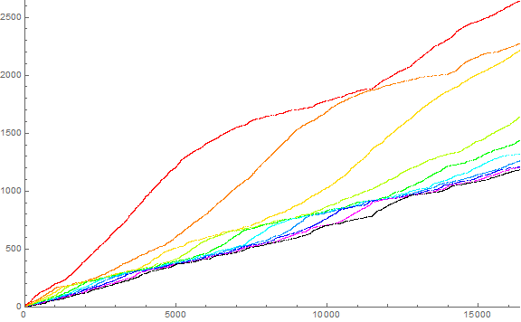
The plot in Figure 4 evokes a notion that the racers are lazy. They muscle off only to at some point gather they have it made, but when the racer in the rear view mirror approaches, seemingly catching them off guard, they hit the gas. In terms of mathematics, we see that the distance x between the d-th and (d+1)-th appearances of m narrow to a certain degree, then suddenly widen again. This is more evident in the enlarged and extended plot. Do we ever see “passes” where one stream crosses another? The non-colorized plot seems to suggest passes happen and the streams do cross, for the sudden “gusto” exhibited by the d-th racer when racer d+1 approaches to seem just about to pass.
Some of the racers seem to pile up after a number of “laps” n. For instance, d = 3 seems to be joined by d = 4 around n = 5500, only to soon after peel off, followed by d = 5, etc., in a sort of wave or linear tangle or “wolf pack”. Is any “passing” going on? The racers d peel off from the wolf pack in order of increasing d; some are freed only to get caught in another wolf pack. Indeed, d = 1 isn’t totally free of the wolf pack; it seemed to have slowed around n = 1000, but sped up before d = 2 slowed and d = 3 caught up. How does the sequence “know” when a racer d should speed up, possibly so as not to have the next car (d + 1) overtake it?
Additionally, we note that the racers d above the dashed line of slope 1/10 appear such that d that are generally above the line are those that tend to be less than the square root of 10.
Passing racers.
We can find the 10 indices where m appears in s, determine their first differences and see if we witness a “pass”.
Table 1 shows the 10 positions n where s(n) = m = t(d, n) is instigated by progenitor d = t(n), for 1 ≤ m ≤ 12 and ignoring the given s(1) = 1:
m | d = racer
lap| 1 2 3 4 5 6 7 8 9 10
---+--------------------------------------------------------
1 | 2 4 6 8 10 12 14 16 18 21
2 | 3 26 28 30 32 35 38 41 45 49
3 | 5 33 43 47 51 55 60 62 64 67
4 | 7 36 56 73 81 86 92 97 105 110
5 | 9 39 61 79 84 91 100 104 107 115
6 | 11 42 65 88 94 96 102 121 130 133
7 | 13 46 69 98 108 122 136 154 167 182
8 | 15 48 72 111 116 131 150 162 179 184
9 | 17 50 77 119 127 134 169 173 180 199
10 | 19 52 80 128 139 142 171 186 190 205
11 | 20 54 82 135 145 164 193 207 209 215
12 | 22 57 85 146 149 170 201 217 222 224
...
If we see the value m equating to “laps” around a “racetrack” and the “racers” designated 0 ≤ d ≤ 9, then n represents their position on the “course”. A “pass” would be the occasion of index n pertaining to column d for a given m proving less than index n for (d + 1) in the same row m. In the first dozen m, we see that the racers maintain their rankings.
Of course, we can replace the positions n with their corresponding d, and find any transposition of d that interrupts the order least to greatest d to find any occasion of “passing”. We take the first differences of these d in row m to identify the “lap” m where the pass happens; any negative first differences would show a “pass”. The dataset of 544297 terms of s accommodates full records for the 10 occurrences of m in s for 1 ≤ m ≤ 45961, and no record of “passing” is seen as of yet.
Challenging racers.
If we do not (yet) observe any “passing”, what is the closest approach or “challenge” of two racers? At the start of the race, with m = 1, the spacing g = 2, meaning we see the term m = 1 at n = 1, even n ≤ 18, and lastly at n = 21. Therefore we have the gaps {2, 2, 2, 2, 2, 2, 2, 3}. From here the gaps tend to grow larger for small d with notable close passes, for instance, g = 2 between d = {5, 6}, at (n, m) = (94, 6), or g = 2 between progenitor digits 8 and 9 starting at (207, 11).
Aside from s(1) = 1 (which is given and thus ignored) and s(2) = 1, we see a single instance of g = 1:
m n_1 n_2 d
-----------------------
15 272 273 8-9
Table 2 lists the positions of 1 ≤ m ≤ 45961 separated by g = 2.
m n_1 n_2 d
-----------------------
1 2 4 1-2
1 4 6 2-3
1 6 8 3-4
1 8 10 4-5
1 10 12 5-6
1 12 14 6-7
1 14 16 7-8
1 16 18 8-9
2 26 28 2-3
2 28 30 3-4
2 30 32 4-5
3 60 62 7-8
3 62 64 8-9
6 94 96 5-6
11 207 209 8-9
12 222 224 9-0
19 368 370 9-0
43 556 558 6-7
62 1068 1070 9-0
187 1466 1468 2-3
188 1470 1472 2-3
308 3647 3649 6-7
Do we see a challenge as close as g = 1 for m > 15, or g = 2 for m > 308? Indeed we might write a sequence of the last-seen g = 1, 2, 3, … for 1 ≤ m ≤ 45961 = {15 (8-9), 308 (6-7), 3404 (3-4), …}, but such only makes sense if we are sure we can never again see such a close challenge as g. We found challenges with g = 4 at m = 45565, and g = 5 at m = 45569, which suggest perhaps that we can expect the same challenges for greater m.
Conjectures regarding s.
We can examine the gaps between incrementation of a given stream d, for instance, we see no term m stemming from d = 1 between s(52) = 21 and s(65) = 22. In the racer analogy, this represents a slow run for d = 1. Obviously, if we see no term m attributable to d = 1 for 52 < n < 65, then certainly other c(d, n) (for d ≠ 1) have been incrementing. Thus, while the stream relating to digit 1 is repressed, the other streams have gained on it. Likewise, when the stream relating to 1 is incrementing often and pulling away from the other streams, they are collectively not able to move forward as fast.
The examination of the behavior of the various streams in the plot is tantamount to examination of the states of the counting functions c(d, n), Indeed, given the progenitor digit d in t(n), we have a single alteration to record and ascribe to a single counting function c(d, n). Therefore, if we were to plot the counting functions only when they severally log a new instance of d in t(n), we would re-create the plot of s(n).
The sequence s is infinite since we can count the number of digits d that appear among the first k digits of s, as we increment k and add 1 to one of the 10 counting functions c(d, n). Since c(d, n) is reported in s as a decimal number and since the counting functions increment by 1 upon each new instance of d in s, we will always be presented with every decimal digit d as n increases; the question merely regards which digit d will set records. This appears to be d = 1.
It seems fair to ascribe the behavior of the counting functions to Benford’s Law, since all the functions begin set to 0 and monotonically increase by 1 whenever t(n) = d. Therefore we conjecture that the counting functions’ behavior is governed by phenomena related to Benford’s Law as s covers many orders of magnitude and, for n > 2, the mean of s(n) exceeds the median of s(n).
The effect of “pole position”.
We have examined trying to best other racers d by selecting a different initial term or terms. Can we find a way to finnagle a win for d ≠ 1? We may set s(1) = 0. In this scenario, c(0, n) > c(d, n) for at least 1 nonzero d for 0 < m < 5. Therefter, d = 0 “beats” d = 9 and sometimes other d as m increases, but never finds itself ahead of d = 1 after m = 1 or d = 2 after m = 2. David Sycamore noted that decimal integers written in standard positional notation cannot begin with 0 so, perhaps d = 0 suffers a sort of disadvantage the other “racers” do not.
Therefore, we used a(1) = 3 or a(1) = 7 with the observed eventuality that these digits tends to “find” their place among the other digits d given enough terms of s, that is, in the order from 1 to 9, followed by 0. We tried beginning the sequence with 7 sevens, only to have d = 7 settle back to its place given enough terms in s. Finally, we tried to overcome the priming of the sequence with the ten digits d by having 22 sevens at the front of the sequence. This did manage to have d = 7 challenge d = 3 but usually rank among d = 5 or d = 6 as n increases. After n = 5000, d = 7 is still out of place, but we surmise that it shall take its place as n increases. Therefore, artificially starting the sequence with anything other than 1 merely results in a delayed organization of the progenitor digits d that yield m in s.
It might be understandable to begin the sequence s with s(0) = 1, but this merely affects the index n and not the general behavior of the sequence.
Changing the number of racers.
We have discussed the case of b = 10 racers, that is, the 10 decimal digits 0 ≤ d ≤ (b − 1). What do “races” resemble given a different number of cars, meaning what does s look like in a different base b? We shall designate sb as the sequence s in base b. Therefore, the variant of s we have studied could also be designated s10. Since we have sb, we likewise can produce the convenient sequence tb of single digits d in in order of appearance in sb.
Binary racers.
The simplest race concerns the binary version of s, i.e., s2. Let s2(1) = 1, s2(n+1) is the number of times the nth bit (binary digit) in the sequence has been seen, up to and including itself. The sequence begins:
1, 1, 2, 3, 1, 4, 5, 6, 7, 2, 3, 8, 4, 9, 10, 11, 5, 12, 13, 14, 15, 6, 16, 17, 18, 7, 8, 9, 19, 10, 11, 20, 12, 13, 21, 22, 14, 23, 15, 24, 16, 25, 26, 27, 17, 28, 29, 30, 18, 19, 31, 32, 20, 33, 34, 35, 36, 21, 37, 38, 39, 40, 41, 42, 22, 43, 23, 24, 25, 26, 44, 27, 28, 29, 45, 46, 30, 31, 47, 32, 48, 49, 50, 51, 33, 34, 35, 52, 36, 37, 53, 54, 38, 39, 55, 56, 57, 40, 58, 41, 59, 42, 60, 61, 62, 43, 63, 44, 45, 64, 65, 46, 47, 66, 67, 48, 68, 69, 49, 70, …
Of course we may see fit to look at s2 in binary; in which case it begins:
1, 1, 10, 11, 1, 100, 101, 110, 111, 10, 11, 1000, 100, 1001, 1010, 1011, 101, 1100, 1101, 1110, 1111, 110, 10000, 10001, 10010, 111, 1000, 1001, 10011, 1010, 1011, 10100, 1100, 1101, 10101, 10110, 1110, 10111, 1111, 11000, 10000, 11001, 11010, 11011, 10001, 11100, 11101, 11110, 10010, 10011, 11111, 100000, 10100, 100001, …
Recall the register c(d, n) for 0 ≤ d ≤ 1 that is the counting function of the number of bits d that have appeared in t2(1..n).
What we have in this case is a sequence that demonstrates the conservation of n = c(0, n) + c(1, n), which follows from the fact that binary digits d can only be either 0 or 1, and if one, the other excluded. Therefore naturally, moves in one bit are reflected in inverse in the other in the plot. As a consequence of binary having 2 digits, we expect to see all terms m > 1 appear precisely twice (and m = 1 thrice).
Clearly, if we were to plot the sum of c(d, n) for all d, we would have a line of slope 1 from (1,1).
Figure 5.2.1 is a plot of s2(n) for 1 ≤ n ≤ 210, showing terms m attributable to d = 1 in red, and d = 0 in blue. We see that this plot exhibits the general slope ½, since n = c(0, n) + c(1, n), even though either function c(d, n) manifests at s2(n) only when t2(n) = d.
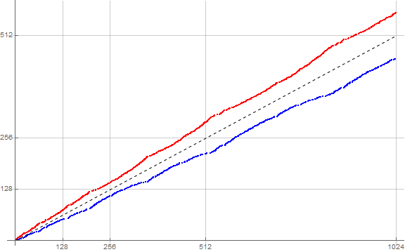
Figure 5.2.2 is a log-log plot of s2(n) for 1 ≤ n ≤ 217, showing terms m attributable to d = 1 in red, and d = 0 in blue.
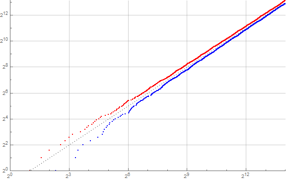
It seems the rate of divergence of c(0, n) and c(1, n) does not scale with n = 2k. We notice that d = 1 enjoys an appreciable advantage up front that it generally sustains.
At any rate, it seems that racer 1 beats racer 0 with very little of the “laziness” or seeming element of surprise and overreaction we see in the decimal case. Instead, it seems that, when racer 1 gets gusto, racer 0 loses spirit, and when racer 0 picks up, racer 1 lulls. This stands to reason, for the “velocity” of the racers d translates into how often digit d appears in t2. When digits d tend to alternate in t2, they track along with the line of slope ½.
Ternary racers.
We examine the ternary case, s3. Let s3(1) = 1, s3(n+1) is the number of times the nth ternary digit in the sequence has been seen, up to and including itself. The sequence begins:
1, 1, 2, 1, 3, 4, 1, 5, 6, 7, 8, 2, 3, 2, 4, 9, 5, 6, 7, 10, 3, 8, 11, 12, 13, 4, 5, 14, 9, 10, 6, 11, 15, 16, 7, 17, 18, 8, 12, 13, 19, 9, 14, 20, 21, 10, 22, 23, 24, 25, 26, 27, 15, 28, 29, 16, 30, 11, 12, 31, 13, 32, 17, 14, 33, 15, 18, 34, 19, 16, 35, 20, 36, 21, 37, 38, 22, 23, 24, 17, 18, 25, 26, 39, 40, 19, 41, 42, 43, 27, 20, 44, 45, 21, 22, 46, 47, 28, 29, 23, 30, 31, 48, 24, 49, 25, 50, 32, 51, 52, 33, 53, 34, 35, 36, 26, 37, 38, 54, 39, …
Of course we may see fit to look at s3 in ternary; in which case it begins:
1, 1, 2, 1, 10, 11, 1, 12, 20, 21, 22, 2, 10, 2, 11, 100, 12, 20, 21, 101, 10, 22, 102, 110, 111, 11, 12, 112, 100, 101, 20, 102, 120, 121, 21, 122, 200, 22, 110, 111, 201, 100, 112, 202, 210, 101, 211, 212, 220, 221, 222, 1000, 120, 1001, 1002, 121, 1010, 102, 110, 1011, 111, 1012, 122, 112, 1020, 120, 200, 1021, 201, 121, 1022, 202, 1100, …
Recall the register c(d, n) for 0 ≤ d ≤ 2 that is the counting function of the number of ternary digits d that have appeared in t3(1..n). What we have in this case is a sequence that demonstrates the conservation of n = c(0, n) + c(1, n) + c(2, n), which follows from the fact that ternary digits d may assume an integer value between 0 and 2 inclusive, and if one, the other two are excluded. Therefore naturally, moves in one digit counting function are reflected in inverse in the sum of the other two. As a consequence of base 3 having as many digits, we expect all m > 1 to appear in the sequence thrice, and m = 1 appearing 4 times.
Figure 5.3.1 is a plot of s3(n) for 1 ≤ n ≤ 37, showing terms m attributable to d = 1 in red, d = 2 in green, and d = 0 in blue. We see that this plot exhibits the general slope 1/3, since n = c(0, n) + c(1, n) + c(2, n), even though only one of the functions c(d, n) manifests at s3(n) only when t3(n) = d.
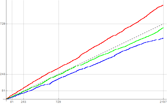
The near-reflection of c(1, n) in red and c(0, n) in blue that we saw for s2 is broken.
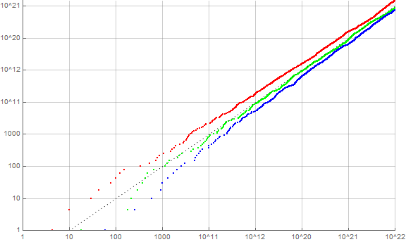
Figure 5.3.2 is a log-log plot of s3(n) for 1 ≤ n ≤ 38, showing terms m attributable to d = 1 in red, d = 2 in green, and d = 0 in blue.
Senary racers.
We visit base b = 6, a base similar to decimal in that it is also a squarefree semiprime. Therefore we are concerned with s6. Let s6(1) = 1, s6(n+1) is the number of times the nth senary digit in the sequence has been seen, up to and including itself. The sequence begins:
1, 1, 2, 1, 3, 1, 4, 1, 5, 1, 6, 7, 1, 8, 9, 10, 11, 2, 12, 2, 13, 2, 14, 2, 3, 4, 2, 5, 6, 15, 7, 8, 9, 10, 3, 3, 11, 3, 16, 3, 12, 4, 17, 18, 19, 13, 20, 5, 21, 4, 6, 7, 22, 4, 8, 14, 5, 9, 15, 4, 6, 16, 5, 10, 5, 11, 23, 17, 24, 12, 18, 6, 13, 14, 7, 25, 6, 26, 27, 15, 8, 9, 28, 19, 20, 21, 7, 29, 16, 22, 17, 10, 30, 7, 23, 11, 8, 31, 12, 9, 32, 10, 18, 11, 24, 12, 13, 8, 25, 9, 19, 10, 33, 11, 26, 34, 27, 28, 35, 36, …
Of course we may see fit to look at s6 in senary; in which case it begins:
1, 1, 2, 1, 3, 1, 4, 1, 5, 1, 10, 11, 1, 12, 13, 14, 15, 2, 20, 2, 21, 2, 22, 2, 3, 4, 2, 5, 10, 23, 11, 12, 13, 14, 3, 3, 15, 3, 24, 3, 20, 4, 25, 30, 31, 21, 32, 5, 33, 4, 10, 11, 34, 4, 12, 22, 5, 13, 23, 4, 10, 24, 5, 14, 5, 15, 35, 25, 40, 20, 30, 10, 21, 22, 11, 41, 10, 42, 43, 23, 12, 13, 44, 31, 32, 33, 11, 45, 24, 34, 25, 14, 50, 11, 35, 15, 12, 51, 20, 13, 52, 14, 30, 15, 40, 20, 21, 12, 41, 13, 31, 14, 53, 15, 42, 54, 43, 44, 55, 100, …
Figure 5.6.1 is a plot of s6(n) for 1 ≤ n ≤ 65, showing terms m attributable to d = 1 in red, ranging through d = 5 in blue and d = 0 in purple. We see that this plot exhibits the general slope 1/6, since n = Sum_{0 ≤ d ≤ 5} c(d, n), even though only one of the functions c(d, n) manifests at s6(n) when t6(n) = d.
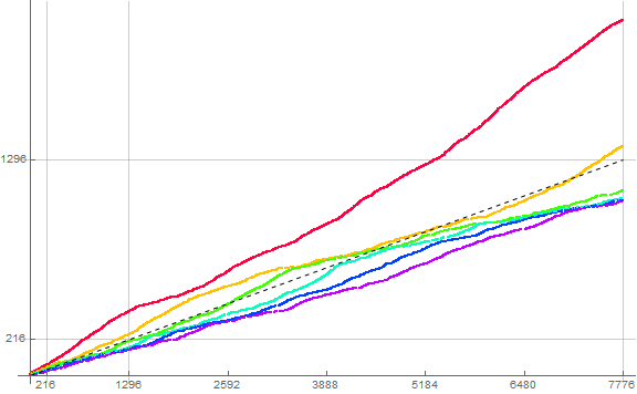
We see 6 vs. 10 “racers”, with m > 1 appearing exactly 6 times in s6, the digits d < 6½ are usually above the line of slope 1/6 from origin. The “racers” in the plot of s6 begins to exhibit the “lazy racer” behavior manifested in the decimal sequence s plotted in Figure 4.
Hexadecimal racers.
Let's look at a base with more digits (and thereby, racers) than b = 10, namely hexadecimal or b = 16. Therefore we are concerned with s16. Let s16(1) = 1, s16(n+1) is the number of times the nth hexadecimal digit in the sequence has been seen, up to and including itself. The sequence begins:
1, 1, 2, 1, 3, 1, 4, 1, 5, 1, 6, 1, 7, 1, 8, 1, 9, 1, 10, 1, 11, 1, 12, 1, 13, 1, 14, 1, 15, 1, 16, 17, 1, 18, 19, 20, 21, 2, 22, 2, 23, 2, 24, 2, 3, 25, 2, 4, 26, 2, 5, 27, 2, 6, 3, 28, 2, 7, 3, 29, 2, 8, 3, 30, 2, 9, 3, 4, 31, 2, 10, 3, 5, 32, 2, 11, 3, 6, 33, 2, 12, 3, 7, 4, 34, 2, 13, 3, 8, 4, 14, 2, 15, 3, 9, 4, 16, 35, 17, 3, 10, 4, 5, 18, 19, 20, 3, 11, 4, 6, 3, 21, 3, 12, 4, 7, 36, 3, 22, 13, …
Of course we may see fit to look at s16 in hexadecimal; in which case it begins:
1, 1, 2, 1, 3, 1, 4, 1, 5, 1, 6, 1, 7, 1, 8, 1, 9, 1, a, 1, b, 1, c, 1, d, 1, e, 1, f, 1, 10, 11, 1, 12, 13, 14, 15, 2, 16, 2, 17, 2, 18, 2, 3, 19, 2, 4, 1a, 2, 5, 1b, 2, 6, 3, 1c, 2, 7, 3, 1d, 2, 8, 3, 1e, 2, 9, 3, 4, 1f, 2, a, 3, 5, 20, 2, b, 3, 6, 21, 2, c, 3, 7, 4, 22, 2, d, 3, 8, 4, e, 2, f, 3, 9, 4, 10, 23, 11, 3, a, 4, 5, 12, 13, 14, 3, b, 4, 6, 3, 15, 3, c, 4, 7, 24, 3, 16, d, …
Here we employ the transdecimal numerals a = 10, b = 11, c = 12, d = 13, e = 14, and f = 15.
Figure 5.16 is a plot of s16(n) for 1 ≤ n ≤ 164, showing terms m attributable to d = 1 in red, ranging through d = 15,with d = 0 in magenta. We see that this plot exhibits the general slope 1/16, since n = Sum_{0 ≤ d ≤ 15} c(d, n), even though only one of the functions c(d, n) manifests at s16(n) when t16(n) = d.
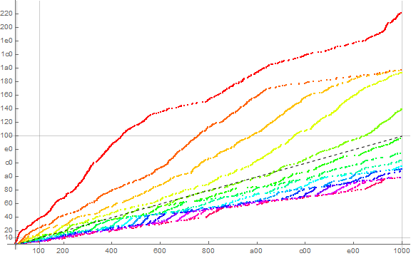
This plot resembles Figure 4, except we have 16 vs. 10 racers, and m > 1 appears precisely 16 times in s16. We see the tangling of racers and their freeing themselves from the wolf pack one by one in turn, in order of d.
Sexagesimal racers.
Finally, we turn to a behemoth base b = 60 used by the ancient Mesopotamians and handily highly composite. It seems certain that divisibility plays no role in the functioning of these sequences, therefore we have arbitrarily selected this familiar large base merely to portray a great number of racers 0 ≤ d ≤ 59.
Therefore we are concerned with s60. Let s60(1) = 1, s60(n+1) is the number of times the nth sexagesimal digit in the sequence has been seen, up to and including itself. The sequence begins:
1, 1, 2, 1, 3, 1, 4, 1, 5, 1, 6, 1, 7, 1, 8, 1, 9, 1, 10, 1, 11, 1, 12, 1, 13, 1, 14, 1, 15, 1, 16, 1, 17, 1, 18, 1, 19, 1, 20, 1, 21, 1, 22, 1, 23, 1, 24, 1, 25, 1, 26, 1, 27, 1, 28, 1, 29, 1, 30, 1, 31, 1, 32, 1, 33, 1, 34, 1, 35, 1, 36, 1, 37, 1, 38, 1, 39, 1, 40, 1, 41, 1, 42, 1, 43, 1, 44, 1, 45, 1, 46, 1, 47, 1, 48, 1, 49, 1, 50, 1, 51, 1, 52, 1, 53, 1, 54, 1, 55, 1, 56, 1, 57, 1, 58, 1, 59, 1, 60, 61, 1, 62, 63, 64, 65, 2, 66, 2, 67, 2, 68, 2, 3, 69, 2, 4, 70, 2, 5, 71, 2, 6, 3, 72, 2, 7, 3, 73, 2, 8, 3, 74, 2, 9, 3, 4, 75, 2, 10, 3, 5, 76, 2, 11, 3, 6, 77, 2, 12, 3, 7, 4, 78, 2, 13, 3, 8, 4, 79, 2, 14, 3, 9, 4, 80, 2, 15, 3, 10, 4, 5, 81, 2, 16, 3, 11, 4, 6, 82, 2, …
Here we note that the priming of the sequence, that is, the introduction of each digit d requires an understandably long range, not complete until n = 59, where we see the priming pattern {1, 1, 2, 1, 3, 1, 4, 1, …, b − 1, 1, b, b+1, 1} manifest, granting an obscene lead for d = 1 in the meantime. The racer d = 1 continues to enjoy a lead as we have the sexagesimal analogy of “teens” (i.e., (b + 1) ≤ m ≤ (2b − 1)) enter the sequence, each introducing the first digit d = 1.
Of course we may see fit to look at s60 in sexagesimal (which may prove far less useful to our eyes); in which case it begins:
1, 1, 2, 1, 3, 1, 4, 1, 5, 1, 6, 1, 7, 1, 8, 1, 9, 1, a, 1, b, 1, c, 1, d, 1, e, 1, f, 1, g, 1, h, 1, i, 1, j, 1, k, 1, l, 1, m, 1, n, 1, o, 1, p, 1, q, 1, r, 1, s, 1, t, 1, u, 1, v, 1, w, 1, x, 1, y, 1, z, 1, A, 1, B, 1, C, 1, D, 1, E, 1, F, 1, G, 1, H, 1, I, 1, J, 1, K, 1, L, 1, M, 1, N, 1, O, 1, P, 1, Q, 1, R, 1, S, 1, T, 1, U, 1, V, 1, W, 1, X, 1, 10, 11, 1, 12, 13, 14, 15, 2, 16, 2, 17, 2, 18, 2, 3, 19, 2, 4, 1a, 2, 5, 1b, 2, 6, 3, 1c, 2, 7, 3, 1d, 2, 8, 3, 1e, 2, 9, 3, 4, 1f, 2, a, 3, 5, 1g, 2, b, 3, 6, 1h, 2, c, 3, 7, 4, 1i, 2, d, 3, 8, 4, 1j, 2, e, 3, 9, 4, 1k, 2, f, 3, a, 4, 5, 1l, 2, g, 3, b, 4, 6, 1m, 2, h, 3, c, 4, 7, 1n, 2, i, 3, d, 4, 8, 5, 1o, 2, j, 3, e, 4, 9, 5, 1p, 2, k, 3, f, 4, a, 5, 1q, 2, l, 3, g, 4, b, 5, 6, 1r, 2, …
Here we employ the transdecimal numerals a = 10, b = 11, c = 12, d = 13, e = 14, …, X = 59.
Because the sequence s60 features so many digits compared to s10, we find that the algorithm is much less fecund, that is, since the compression offered by base 60 is greater than that of decimal, we see numbers expressed with fewer sexagesimal digits, therefore we have fewer terms given the same number of iterations of the respective algorithms.
Figure 5.60 is a plot of s60(n) for 1 ≤ n ≤ 602, showing terms m in a color function that sets d = 1 to red, ranging through d = 59,with d = 0 in magenta-red. We see that this plot exhibits the general slope 1/60, since n = Sum_{0 ≤ d ≤ 59} c(d, n), even though only one of the functions c(d, n) manifests at s60(n) when t60(n) = d. Due to the difficulty in discerning the lines, we present an enlarged plot of s60(n) for 1 ≤ n ≤ 603 at this link.
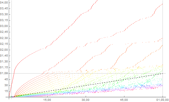
It seems that the plot of s60 presents many of the same features as we see in s.
This paper is a work in progress that may be appended as we continue observing the lazy racer sequence s.
Afterword.
In examining the OEIS to input the data 16 September 2021, D. Sycamore came to find A332182 had already been entered by Rémy Sigrist on 30 November 2018. Therefore, despite having arrived at the idea independently, the original notion attributes to Rémy Sigrist.
Appendix:
Code 1: Generate s(n) and create t(n), the n-th digit d in s:
s = Block[{a = {1}, s},
Array[Set[ s[Mod[#, 10] ], 0] &, 10];
Do[Map[(s[#]++; AppendTo[a, s[#]]) &,
IntegerDigits@ a[[i]] ], {i, 2^10}]; a ];
t = Flatten@ IntegerDigits[s];
Code 2: Plot s(n) to generate Figure 2. To label for a plot like Figure 3, change Labeled[#2, #2] to Labeled[#2, #3].
Block[{c},
c = {Red, Orange, Hue[1/7], Hue[3/14], Green, Hue[1/2], Hue[4/7], Blue, Hue[5/6], Black};
ListPlot[
Array[Style[Labeled[#2, #2], c[[#3 /. 0 -> 10]]] & @@
{#, s[[#]], t[[If[# == 1, 1, # - 1]]]} &, 120],
ImageSize -> Large, GridLines -> Automatic, PlotStyle -> PointSize[Medium]] ]]
Array[Prepend[Position[s, #][[All, 1]], #] &, 12] // TableForm
Concerns OEIS sequences:
A322182: s(n).
Document Revision Record.
2020 1221 1530 Created.
2020 1224 0930 Addition of racers in other bases.
2021 0916 1745 Citation of Rémy Sigrist’s A322182.