Self-referential counting sequences.
Written by Michael Thomas De Vlieger, St. Louis, Missouri, 2021 0118.
Abstract.
We examine simple self-referential sequences that apply a basic number-theoretical counting function f(n) = k to the previous term m and return the number c of terms in the sequence that have the same value k. The sequences produce a plot that has various trajectories k, only one of which is active for a given n; whenever trajectory k is active, c increments. Despite the simplicity of the definition, there arises a measure of gentle complexity that seems to resolve to an aggregate order for large n.
Introduction.
Number theoretical counting functions have been known since antiquity, enumerating entities of interest to the first mathematicians. Whereupon these thinkers constructed concepts such as prime numbers and divisors, they thought to count the number of such entities for a given number n. The divisor counting function τ(n) = OEIS A5(n), yields the number of d | n, that is, a whole number d such that another whole number d' can be found to produce n = d × d'. Another example is the (big) Omega function Ω(n) = A1222(n), the number of prime divisors p | n, with multiplicity, such that Ω(12) = 3, since 12 = 2 × 2 × 3. This, as opposed to the (little) omega function ω(n) = A1221(n), the number of distinct prime divisors p | n; here ω(12) = 2, since 12 = 2² × 3, and there are only two distinct primes; 2 is squared and thus counted only once. (The little omega function is sometimes called ν(n).) Generally, we regard basic number theoretical counting functions f(n) = k for their conceptual simplicity.
Herein we are interested in kicking off an integer sequence S(n) = m with a simple initial term, then we apply f(m) → k. How many k have we seen hitherto? We enumerate distinct k with a new register ck, reporting these whenever f(S(n−1)) = k.
We shall examine the divisor counting function τ(n) and the big omega function Ω(n) among other elementary number-theroretical counting functions in the context of such a self-referential counting sequence or SRCS S(n). In all cases, it seems appropriate to start each off with the empty product 1, as these elementary number theoretical counting functions have to do with multiplication.
The self-referential tau counting sequence.
Let s(1) = 1, therefter s(n+1) = ck, the number of instances of k = τ(s(n)) present in the sequence for 1 ≤ n.[1]
The sequence begins:
1, 1, 2, 1, 3, 2, 3, 4, 1, 4, 2, 5, 6, 1, 5, 7, 8, 2, 9, 3, 10, 3, 11, 12, 1, 6, 4, 4, 5, 13, 14, 5, 15, 6, 7, 16, 1, 7, 17, 18, 2, 19, 20, 3, 21, 8, 9, 6, 10, 11, 22, 12, 4, 7, 23, 24, 1, 8, 13, 25, 8, 14, 15, 16, 2, 26, 17, 27, 18, 5, 28, 6, 19, 29, 30, 2, 31, 32, 7, 33, 20, 8, 21, 22, 23, 34, 24, 3, 35, 25, 9, 10, 26, 27, 28, 9, 11, 36, 1, 9, 12, 10, 29, 37, 38, 30, 4, 13, 39, 31, 40, 5, ...
Code 1.1 generates the sequence.
Examples:
s(2) = 1 since τ(s(1)) = k = 1 has appeared once in s. (The number 1 has 1 divisor, 1).
s(3) = 2 since τ(s(2)) = k = 1 has appeared twice in s.
s(4) = 1 since τ(s(3)) = k = 2 has appeared once in s.
s(5) = 3 since k = 1 has appeared thrice in s.
s(6) = 2 since k = 2 has appeared twice in s, etc.
We note that a second, sidecar sequence s'(n) might track the values m found in s. This auxiliary sequence is simply the mappings τ(n) across m in s(n). Code 1.2 generates the sequence.The first terms in s'(n) are:
0, 1, 1, 2, 1, 2, 2, 2, 3, 1, 3, 2, 2, 4, 1, 2, 2, 4, 2, 3, 2, 4, 2, 2, 6, 1, 4, 3, 3, 2, 2, 4, 2, 4, 4, 2, 5, 1, 2, 2, 6, 2, 2, 6, 2, 4, 4, 3, 4, 4, 2, 4, 6, 3, 2, 2, 8, 1, 4, 2, 3, 4, 4, 4, 5, 2, 4, 2, 4, 6, 2, 6, 4, 2, 2, 8, ...
This sequence registers the values τ(m) = k (We start this sequence with 0 as a placeholder by definition, since s(1) = 1 is given). Furthermore, we may take the union of s' = K so as to determine the distinct k taken by s. We anticipate that all the natural numbers are in K. In the snippet of data above, we see that 1 ≤ k ≤ 6 and k = 8 are in K thus far and ignoring k = 0. We find that prime k tend to emerge late as k increases. We attribute the reluctance of prime k to appear in s to the fact that only τ(pe) is prime only for p and e prime.
Crucially, we note that k = 1 arises only for m = 1, since 1 is the only number with 1 divisor. Hence, we might use the occasion of k = 1 in the sequence s' to herald the appearance at s'(n−1) of a hitherto unseen value of k.
Figure 1.1 is a plot of (n, s(n)) for 1 < n < 120, color coded and many points labeled as to the value of k so as to identify the trajectories.
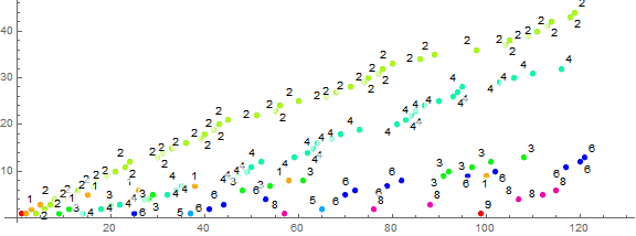
Again, for a given trajectory k, we see incrementation of ck whenever same registers in s. There is a sorting as to k, hence, those k that might be produced by multiple prime signatures F in A025487 have accelerated trajectories in s. In other words, the acceleration of trajectory k varies according to A1055(k). For small n, s(n) = m prime fairly often, since 2, 3, 5, 7, etc. instances are prime and have τ(m) = 2. We see 4, 9, and eventually, 25 instances producing τ(m) = 3, which aren’t nearly as prone to entering s as a small prime m.
Figure 1.2 is a log-log plot of (n, s(n)) for 1 < n < 216 using a color function to represent k. (See Code 1.3)
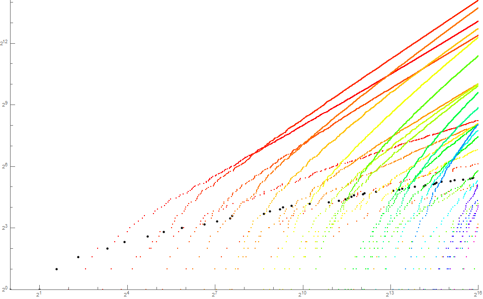
We see the crossing of trajectories, some rather early such as c2(n) > c1(n) for n ≥ 8, c4(n) > c2(n) for n ≥ 309 and c8(n) > c2(n) for n ≥ 7571. Further we can see c8(n) > c6(n) for n ≥ 1020 and c12(n) > c6(n) for n ≥ 17186.
Hence it seems we see some facsimile of k > 1 in A033833 (i.e., 4, 8, 12, 16, 24, 36, 48, 72, 96, 120, 144, 192, 216, 240, 288, 360, …) with the maximum acceleration.
The self-referential regular counting sequence.
Naturally we’d like to examine a self-referential sigma counting sequence, based upon the function σ(n), the divisor sum function. This function is not a counting function itself but a summatory function, and its behavior perhaps departs out of scope from the self-referential counting sequences that are based themselves upon number theoretical counting sequences. We furnish plots of such a sequence r(n) in the Appendix. [4]
Let the “regular counting function” rcf(n) = A010846(n) be the number of 1 ≤ j ≤ n such that j | ne for e ≥ 0. We note such j | ne are divisors when e ≤ 1, otherwise we call j “semidivisors” or “quasidivisors”. Hence, rcf(n) > τ(n), but for n such that ω(n) ≤ 1, rcf(n) = τ(n). Code 2.0 most efficiently calculates rcf(n) for large n.
Example: n = 10 has 4 divisors {1, 2, 5, 10} but additionally 4 | 10² and 8 | 10³, thus rcf(10) = 6.
Example: n = 12 has 6 divisors {1, 2, 3, 4, 6, 12} but additionally 8 | 12² and 9 | 12², thus rcf(12) = 8.
The term “regular counting function” derives from the terminology “regular” pertaining to base b denominators j that produce terminating expansions. In a manner analogous to the highly composite numbers A2182 being those numbers that set records for the divisor counting function τ(n), we have the highly regular numbers A244052 that set records for the regular counting function rcf(n). The divisor counting function is naturally bound, as no d | n exceeds n, while we can identify regular j | ne that exceed n, an obvious example being n² | n². Therefore there is a bound effect on rcf(n) that does not occur for τ(n). Without the bound n, we see an infinity of regular numbers j | ne for n > 1. Therefore we use this more obscure number theoretical function as the basis for a new self-referential counting sequence.
Then t(1) = 1, therefter t(n+1) = ck, the number of instances of k = rcf(u(n)) present in the sequence for 1 ≤ n.
The sequence begins:
1, 1, 2, 1, 3, 2, 3, 4, 1, 4, 2, 5, 6, 1, 5, 7, 8, 1, 6, 2, 9, 3, 10, 1, 7, 11, 12, 1, 8, 2, 13, 14, 2, 15, 3, 16, 4, 4, 5, 17, 18, 1, 9, 6, 5, 19, 20, 2, 21, 6, 7, 22, 1, 10, 3, 23, 24, 1, 11, 25, 7, 26, 2, 27, 3, 28, 3, 29, 30, ...
Code 2.1 generates the sequence.
Examples:
t(2) = 1 since rcf(t(1)) = k = 1 has appeared once in s. (The number 1 has 1 regular number, 1).
t(3) = 2 since rcf(t(2)) = k = 1 has appeared twice in s.
t(4) = 1 since rcf(t(3)) = k = 2 has appeared once in s. (For primes p, rcf(p) = τ(p) = 2).
t(5) = 3 since k = 1 has appeared thrice in t.
t(6) = 2 since k = 2 has appeared twice in t, etc.
This sequence departs from s(n) for n > 17.
We note that a second, sidecar sequence t'(n) might track the values m found in t. This auxiliary sequence is simply the mappings rcf(n) across m in t(n). Code 2.2 generates the sequence. The first terms in t'(n) are:
0, 1, 1, 2, 1, 2, 2, 2, 3, 1, 3, 2, 2, 5, 1, 2, 2, 4, 1, 5, 2, 3, 2, 6, 1, 2, 2, 8, 1, 4, 2, 2, 6, 2, 5, 2, 5, 3, 3, 2, 2, 10, 1, 3, 5, 2, 2, 8, 2, 5, 5, 2, 7, 1, 6, 2, 2, 11, 1, 2, 3, 2, 7, 2, 4, 2, 8, 2, 2, 18, 1, 8, 3, 4, 3, 3, 6, ...
This sequence registers the values rcf(m) = k (We start this sequence with 0 as a placeholder by definition, since t(1) = 1 is given). Furthermore, we may take the union of t' = K so as to determine the distinct k taken by t. We anticipate that all the natural numbers are in K. In the snippet of data above, we see that {1, 2, 3, 4, 5, 6, 7, 8, 10, 11, 18} are in K thus far and ignoring k = 0. Here we find that 9 is more reluctant to enter the sequence than is 11, and 18 is present since rcf(30) = 18, and generally, numbers k in A244053 appear early.
Crucially, we note that k = 1 arises only for m = 1, since 1 is the only number with 1 regular number. Hence, we might use the occasion of k = 1 in the sequence s' to herald the appearance at t'(n−1) of a hitherto unseen value of k.
Figure 2.1 is a plot of (n, t(n)) for 1 < n < 120, color coded and many points labeled as to the value of k so as to identify the trajectories.
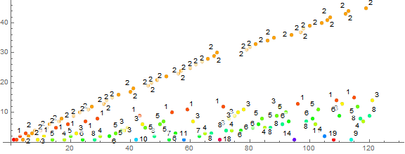
The plot resembles that in Figure 1.1 pertaining to the divisor counting function, except that the k tend to be larger than same for s(n). The trajectory k = 2 pertains to primes as it does in s(n), and the trajectory k = 5 to squarefree semiprimes (since, for n = pq where p and q are dissimilar primes and p < q, n > p² and p² | n²). The trajectory k = 3 pertains to squares of primes, since 1 | p | p². For s(n), the trajectory k = 4 instead pertains to squarefree semiprimes. Because of the effect of the bound n on rcf(n), it is harder to generalize k to a given set of prime signatures as is same for the divisor counting function.
Figure 2.2 is a log-log plot of (n, t(n)) for 1 < n < 216 using a color function to represent k. (See Code 2.3)
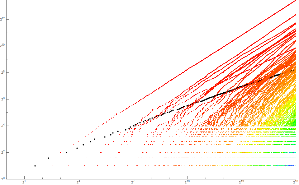
Figure 2.2 resembles Figure 1.2 in part, however we see far more trajectories in t(n), since a number m of a given prime signature yields different values k = rcf(m) on account of the effect of the bound on an infinite sequence of regular j | ne.
The self-referential big Omega counting sequence.
Let u(1) = 1, therefter u(n+1) = ck, the number of instances of k = Ω(u(n)) present in the sequence for 1 ≤ n.[2]
The sequence begins:
1, 1, 2, 1, 3, 2, 3, 4, 1, 4, 2, 5, 6, 3, 7, 8, 1, 5, 9, 4, 5, 10, 6, 7, 11, 12, 2, 13, 14, 8, 3, 15, 9, 10, 11, 16, 1, 6, 12, 4, 13, 17, 18, 5, 19, 20, 6, 14, 15, 16, 2, 21, 17, 22, 18, 7, 23, 24, 3, 25, 19, 26, 20, 8, 9, 21, 22, 23, 27, 10, 24, 4, 25, 26, 27, 11, 28, 12, 13, 29, 30, 14, 28, 15, 29, 31, 32, 1, 7, 33, 30, 16, 5, 34, 31, 35, 32, 2, 36, 6, 33, 34, 35, 36, 7, 37, 38, 37, 39, 38, 39, ...
Code 3.1 generates the sequence.
Examples:
u(2) = 1 since Ω(u(1)) = k = 0 has appeared once in u. (The number 1 has 1 divisor, 1).
u(3) = 2 since Ω(u(2)) = k = 0 has appeared twice in u.
u(4) = 1 since Ω(u(3)) = k = 1 has appeared once in u.
u(5) = 3 since k = 0 has appeared thrice in u.
u(6) = 2 since k = 1 has appeared twice in u, etc.
The sequence u is the same as s for 1 ≤ n ≤ 13.
We can define an auxiliary sequence u'(n) might track the values m found in u. This auxiliary sequence is simply the mappings Ω(n) across m in u(n). Code 3.2 generates the sequence.The first terms in u'(n) are:
0, 0, 0, 1, 0, 1, 1, 1, 2, 0, 2, 1, 1, 2, 1, 1, 3, 0, 1, 2, 2, 1, 2, 2, 1, 1, 3, 1, 1, 2, 3, 1, 2, 2, 2, 1, 4, 0, 2, 3, 2, 1, 1, 3, 1, 1, 3, 2, 2, 2, 4, 1, 2, 1, 2, 3, 1, 1, 4, 1, 2, 1, 2, 3, 3, 2, 2, 2, 1, 3, 2, 4, 2, 2, 2, 3, 1, 3, 3, 1, 1, 3, 2, 3, 2, 1, 1, 5, 0, 1, 2, 3, 4, 1, ...
This sequence registers the values Ω(m) = k (We start this sequence with 0 as a placeholder by definition, since u(1) = 1 is given). Furthermore, we may take the union of u' = K so as to determine the distinct k taken by u. We anticipate that all the natural numbers are in K and in the case of u', it seems even more plausible than s' for the fact that K accretes incrementally rather than in the fashion of the union of u', which favors numbers in A1105. We can form an arbitrary n by taking the product of any number of primes (here, we consider primes with multiplicity). Given the definition of the sequence and the nature of the registers ck that increment upon the emergence of a new instance of k, through induction we know that all natural numbers will appear in the registers, thus, all values of k appear in u'.
In the snippet of data above, we see that 0 ≤ k ≤ 5 are in K thus far.
Crucially, we note that k = 0 arises only for m = 1, since 1 is the empty product. Hence, we might use the occasion of k = 0 in the sequence u' to herald the appearance at u'(n−1) of a hitherto unseen value of k.
Figure 3.1 is a plot of (n, u(n)) for 1 < n < 120, color coded and many points labeled as to the value of k so as to identify the trajectories.
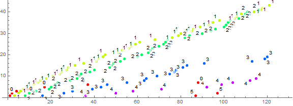
Figure 3.1 shows k = 0 (thus, previous terms m = 1) dominant but quickly surpassed by the trajectory k = 1 that pertains to primes. We see the crossing of trajectories, some rather early such as c1(n) > c0(n) for n ≥ 6, c2(n) > c1(n) for n ≥ 74 and c3(n) > c2(n) for n ≥ 109776. It seems that c(k+1) crosses ck at some n. This is borne out by Figure 3.2.
Figure 3.2 is a log-log plot of (n, u(n)) for 1 < n < 217 using a color function to represent k. (See Code 3.3):
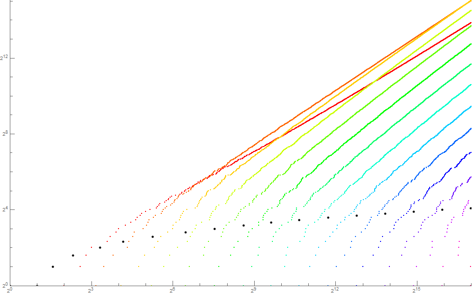
Compared to Figure 1.2, this plot seems to exhibit a more exponentially regular introduction of incremented, novel k as n increases. The behavior of the trajectories seems to be similar for all k, with the declining slope most pronounced for small k.
The self-referential little omega counting sequence.
We might consider a variant of sequence u. Let v(1) = 1, therefter v(n+1) = ck, the number of instances of k = ω(v(n)) present in the sequence for 1 ≤ n.
The sequence begins:
1, 1, 2, 1, 3, 2, 3, 4, 5, 6, 1, 4, 7, 8, 9, 10, 2, 11, 12, 3, 13, 14, 4, 15, 5, 16, 17, 18, 6, 7, 19, 20, 8, 21, 9, 22, 10, 11, 23, 24, 12, 13, 25, 26, 14, 15, 16, 27, 28, 17, 29, 30, 1, 5, 31, 32, 33, 18, 19, 34, 20, 21, 22, 23, 35, 24, 25, 36, 26, 27, 37, 38, 28, 29, 39, 30, 2, 40, 31, 41, 42, 3, 43, 44, 32, 45, 33, 34, 35, 36, 37, 46, 38, 39, 40, 41, 47, 48, 42, 4, 49, 50, 43, 51, ...
Code 4.1 generates the sequence.
Examples:
v(2) = 1 since ω(v(1)) = k = 0 has appeared once in v. (The number 1 has 1 divisor, 1).
v(3) = 2 since ω(v(2)) = k = 0 has appeared twice in v.
v(4) = 1 since ω(v(3)) = k = 1 has appeared once in v.
v(5) = 3 since k = 0 has appeared thrice in v.
v(6) = 2 since k = 1 has appeared twice in v, etc.
The sequence v is the same as u for 1 ≤ n ≤ 8.
We can define an auxiliary sequence v'(n) might track the values m found in v. This auxiliary sequence is simply the mappings ω(n) across m in v(n). Code 4.2 generates the sequence.The first terms in v'(n) are:
0, 0, 0, 1, 0, 1, 1, 1, 1, 1, 2, 0, 1, 1, 1, 1, 2, 1, 1, 2, 1, 1, 2, 1, 2, 1, 1, 1, 2, 2, 1, 1, 2, 1, 2, 1, 2, 2, 1, 1, 2, 2, 1, 1, 2, 2, 2, 1, 1, 2, 1, 1, 3, 0, 1, 1, 1, 2, 2, 1, 2, 2, 2, 2, 1, 2, 2, 1, 2, 2, 1, 1, 2, 2, 1, 2, 3, 1, 2, 1, 1, 3, 1, 1, 2, 1, 2, 2, 2, 2, 2, 1, 2, 2, 2, 2, 1, 1, 2, 3, 1, 1, 2, 1, 2, 2, 2, 2, 1, 2, 2, 1, 1, 2, 2, 2, 2, 1, 2, 2, ...
This sequence registers the values ω(m) = k (We start this sequence with 0 as a placeholder by definition, since v(1) = 1 is given). Furthermore, we may take the union of v' = K so as to determine the distinct k taken by v. We anticipate that all the natural numbers are in K and in the case of v' for the same reasons stated for sequence u'; we can form an arbitrary n by taking the product of any number of primes (here, we consider distinct primes).
Once again, k = 0 arises only for m = 1, since 1 is the empty product. Hence, we might use the occasion of k = 0 in the sequence v' to herald the appearance at v'(n−1) of a hitherto unseen value of k.
Figure 4.1 is a plot of (n, v(n)) for 1 < n < 120, color coded and many points labeled as to the value of k so as to identify the trajectories.
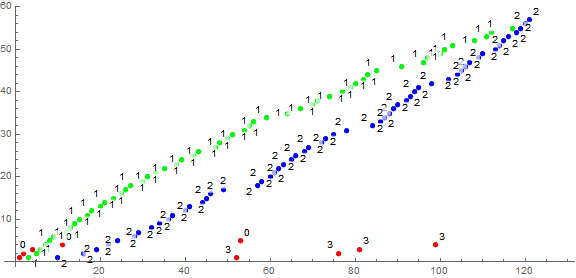
It is apparent that v(n) is simpler than u(n) as ω(m) < Ω(m) for n that are not squarefree.
Figure 4.2 is a log-log plot of (n, v(n)) for 1 < n < 218 using a color function to represent k. (See Code 4.3):
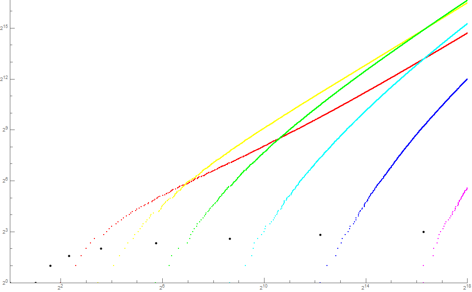
Once again this plot is simpler than Figure 3.2, yet we observe the same apparent increasingly delayed maturation process for trajectory k as k increases. We see the crossing of trajectories, some rather early such as c1(n) > c0(n) for n ≥ 7, c2(n) > c1(n) for n ≥ 119 and c3(n) > c2(n) for n ≥ 85739. It seems that c(k+1) crosses ck at some n, just as seen in the plot in Figure 3.2 of u(n).
The self-referential Möbius sequence.
Let w(1) = 1, therefter w(n+1) = ck, the number of instances of k = μ(w(n)) present in the sequence for 1 ≤ n. Recall that the Möbius function μ(1) = 1; μ(n) = (−1)k for n is the product of k different primes; otherwise μ(n) = 0. Hence −1 ≤ k ≤ 1. As a convention to handle zeros, if w(n) = 0, then k = 0.
The sequence begins:
1, 1, 2, 1, 3, 2, 3, 4, 1, 4, 2, 5, 6, 5, 7, 8, 3, 9, 4, 5, 10, 6, 7, 11, 12, 6, 8, 7, 13, 14, 9, 8, 9, 10, 10, 11, 15, 12, 11, 16, 12, 13, 17, 18, 14, 13, 19, 20, 15, 14, 15, 16, 16, 17, 21, 17, 22, 18, 18, \
19, 23, 24, 20, 21, 19, 25, 22, 20, 23, 26, 21, 22, 23, 27, 24, 25, 26, 24, 27, 28, ...
Code 5.1 generates the sequence.
Examples:
w(2) = 1 since μ(w(1)) = k = 1 has appeared once in w.
w(3) = 2 since μ(w(2)) = k = 1 has appeared twice in w.
w(4) = 1 since μ(w(3)) = k = −1 has appeared once in w.
w(5) = 3 since k = 1 has appeared thrice in w.
w(6) = 2 since k = −1 has appeared twice in w, etc.
We can define an auxiliary sequence w'(n) might track the values m found in w. This auxiliary sequence is simply the mappings μ(n) across m in w(n). Code 5.2 generates the sequence.The first terms in w'(n) are:
0, 1, 1, -1, 1, -1, -1, -1, 0, 1, 0, -1, -1, 1, -1, -1, 0, -1, 0, 0, -1, 1, 1, -1, -1, 0, 1, 0, -1, -1, 1, 0, 0, 0, 1, 1, -1, 1, 0, -1, 0, 0, -1, -1, 0, 1, -1, -1, 0, 1, 1, 1, 0, 0, -1, 1, -1, 1, 0, 0, -1, -1, 0, 0, 1, -1, 0, 1, 0, -1, 1, 1, 1, -1, 0, 0, 0, 1, 0, 0, 0, -1, 0, -1, -1, -1, -1, 0, -1, 1, 0, 0, 1, 1, 0, 1, 0, 1, -1, 1, ...
This sequence registers the values μ(m) = k (We start this sequence with 0 as a placeholder by definition, since μ(1) = 1 is given).
Figure 5.1 is a plot of (n, w(n)) for 1 < n < 120, color coded and many points labeled as to the value of k so as to identify the trajectories.

The sequence seems to hold k = ±1 nearly equal and k = 0 predominant as n increases, with c0/c1 ≈ 1.289.
Figure 5.2 is a log-log plot of (n, w(n)) for 1 < n < 216 using a color function to represent k. (See Code 5.3):

The sequence w is an example of SRCS based upon a function that has a finite range of values k.
Conclusion.
We have examined the self-referential counting sequences (SRCS) based upon select multiplicative elementary number-theoretical counting functions, selecting 3 well-known functions and 1 function that introduces the effect of the bound of n. In all the studied sequences, the value k = f(m) for previous term m assumes a trajectory k evident in the plot of the SRCS. The register ck increments whenever a new instance of k arises, and then enters the sequence as the current term. These trajectories can be ascribed to the multiplicative nature of the previous term m. The trajectories k are seen to waver for small ck but tend to assume a more crisply defined plot.
We studied the divisor counting function τ(n) via SRCS s and the regular counting function rcf(n) via t, seeing as the divisor d | n is a special case of a regular number j | ne. In sequence s, the trajectories k seem to accelerate based on A1055(k), with those k in A033833 enjoying maximum acceleration. The variant t exhibits a more complex behavior.
The big and little omega functions were the subject of study via SRCS u and v, respectively, the latter with a simpler plot. The trajectories k exhibited cleaner and more well defined curve-like paths in a quasi-regular exponential pitch. We forward a conjecture in both cases that suggests that the trajectory (k+1) crosses that of k at some n.
The Möbius SRCS w is one example of such a sequence where the range of k is finite, constrained to 3 possible values. The plot settles into three trajectories where k = ±1 are more or less (but not exactly) equal, and trajectory 0 is approximately 1.289 times either of the others as n increases. The trajectories have slope of 1/3, as each ck may only increment when activated by μ(m).
The self-referential counting sequence presents an interesting take on the basis function f(n), arranging its terms m in trajectories k that sort out according to the commonness of the value k amid the possible values of f(n).
Appendix:
I would like to acknowledge David J. Sycamore of Megavissey, England for ideas regarding sundry sequences, including two of these. I would also like to acknowledge the editors of the Online Encyclopedia of Integer Sequences (OEIS), a ready resource for all mathematics and brilliant product of Dr. Neil J. A. Sloane. Thank you.
Notes:
[1] The tau SRCS is provisionally designated S20210114 and was posed by David Sycamore in personal correspondence received 14 January 2021.
[2] The big Omega SRCS is provisionally designated S20210115 and was posed by David Sycamore in personal correspondence received 14 January 2021.
[3] Furthermore, t(n) is designated S20210118, v(n) as S20210119, w(n) as S20210121, while the sequence based upon σ(n) is designated S20210113.
[4] Plots of SRCS based upon σ(n): Let s(1) = 1, therefter s(n+1) = ck, the number of instances of k = σ(s(n)) present in the sequence for 1 ≤ n.
Figure 6.1 is a plot of (n, r(n)) for 1 < n < 120, color coded and many points labeled as to the value of k so as to identify the trajectories. Generate r(n) via Code 6.1, and the sidecar sequence r'(n) via Code 6.2.
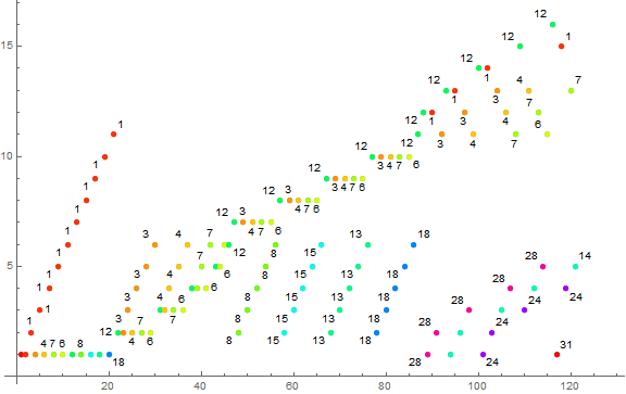
Figure 6.2 is a log-log plot of (n, r(n)) for 1 < n < 214 using a color function to represent k. See Code 6.3.
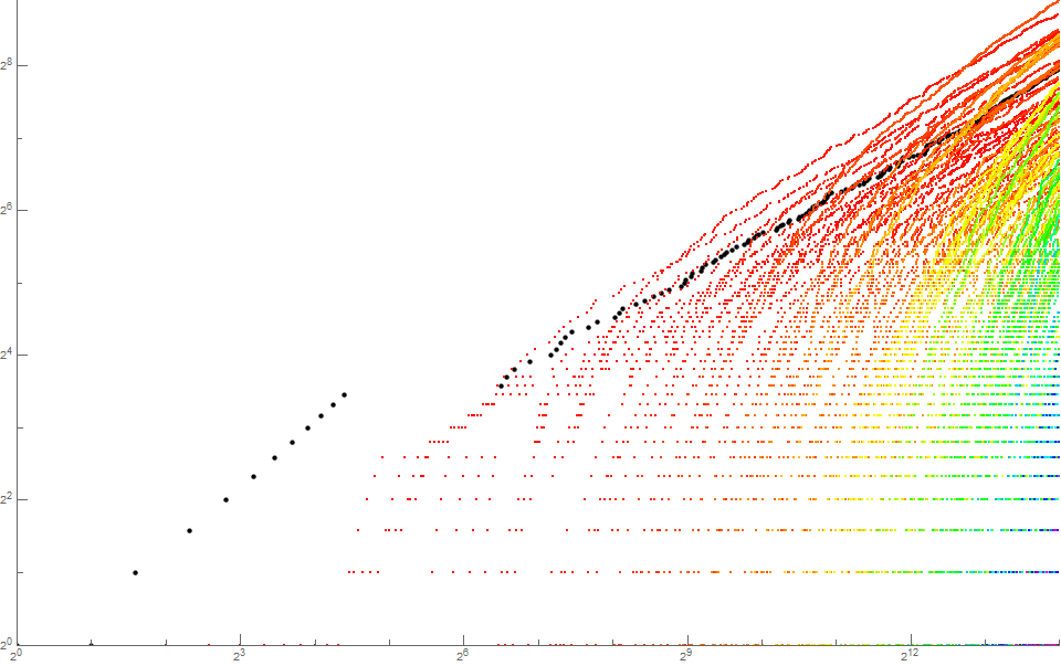
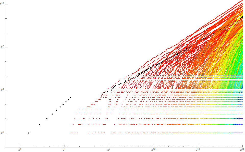
Figure 6.3 is a log-log plot of (n, r(n)) for 1 < n < 216 using a color function to represent k. (The trajectories of some k are effaced by those of larger k due to the placement of their points later in the plot generation process).
Code 1.1: Generate the first 120 terms m in s(n):
Block[{a = {1}, c}, c[0] = 1;
Do[(If[! IntegerQ@ c[#], Set[c[#], 1], c[#]++];
AppendTo[a, c[#]]) &@
DivisorSigma[0, a[[-1]]];, 120]; a]
This code generates 10000 terms in under a second, 105 terms in a quarter minute, and a million terms in about 120 minutes.
Code 1.2: Generate the first 120 terms k in s'(n):
Block[{a = {1}, b = {0}, c, m}, c[0] = 1;
Do[(If[! IntegerQ@ c[#], Set[c[#], 1], c[#]++];
AppendTo[a, c[#]]; AppendTo[b, #]) &@
DivisorSigma[0, a[[-1]]], 120]; b]
Code 1.3: Generate and plot s(n) and use a color algorithm to accentuate trajectories k as seen in Figure 1.2:
Block[{nn = 2^16, c, m, r, s = {1}, t = {0}, u, out = -2^8},
Do[(If[! IntegerQ@ c[#], Set[c[#], 1], c[#]++];
AppendTo[s, c[#]]; AppendTo[t, #]) &@
DivisorSigma[0, s[[-1]]];, 120]
m = Max[t]; u = Union@ t;
Map[Set[r[#], ReplacePart[ConstantArray[out, Length[t] ],
Map[# -> s[[#]] &, Position[t, #][[All, 1]]]]] &, u];
ListPlot[Map[r[#] &, u], ImageSize -> 960,
ScalingFunctions -> {"Log2", "Log2"},
PlotRange -> {{1, Length@ s}, {1, Max@ s}},
PlotStyle -> Map[Directive[{PointSize[If[# <= 1, Medium, Small]],
If[# <= 1, Black, Hue[(# - 2)/m]]}] &, u]]]
Code 2.0: Most efficient code that yields rcf(n):
rcf[1] = 1;
rcf[n_] :=
Function[w,
ToExpression@
StringJoin["Module[{n = ", ToString@ n,
", k = 0}, Flatten@ Table[k++, ",
Most@ Flatten@ Map[{#, ", "} &, #], "]; k]"] &@
MapIndexed[
Function[p,
StringJoin["{", ToString@ Last@ p, ", 0, Log[",
ToString@ First@ p, ", n/(",
ToString@
InputForm[
Times @@ Map[Power @@ # &, Take[w, First@ #2 - 1]]],
")]}"]]@ w[[First@ #2]] &, w]
]@ Map[{#, ToExpression["p" <> ToString@ PrimePi@ #]} &,
FactorInteger[n][[All, 1]] ]
Code 2.1: Generate the first 120 terms m in t(n) using Code 2.0:
Block[{a = {1}, c}, c[0] = 1;
Do[(If[! IntegerQ@ c[#], Set[c[#], 1], c[#]++];
AppendTo[a, c[#]]) &@
rcf[a[[-1]]];, 120]; a]
This code generates 10000 terms in under a second, 105 terms in a quarter minute, and a million terms in about 120 minutes.
Code 2.2: Generate the first 120 terms k in t'(n) using Code 2.0:
Block[{a = {1}, b = {0}, c, m}, c[0] = 1;
Do[(If[! IntegerQ@ c[#], Set[c[#], 1], c[#]++];
AppendTo[a, c[#]]; AppendTo[b, #]) &@
rcf[a[[-1]]], 120]; b]
Code 2.3: Generate and plot t(n) and use a color algorithm to accentuate trajectories k as seen in Figure 2.2, requires Code 2.0:
Block[{nn = 2^14, c, m, r, s = {1}, t = {0}, u, out = -2^8},
Do[(If[! IntegerQ@ c[#], Set[c[#], 1], c[#]++];
AppendTo[s, c[#]]; AppendTo[t, #]) &@
rcf[s[[-1]]];, 120]
m = Max[t]; u = Union@ t;
Map[Set[r[#], ReplacePart[ConstantArray[out, Length[t] ],
Map[# -> s[[#]] &, Position[t, #][[All, 1]]]]] &, u];
ListPlot[Map[r[#] &, u], ImageSize -> 960,
ScalingFunctions -> {"Log2", "Log2"},
PlotRange -> {{1, Length@ s}, {1, Max@ s}},
PlotStyle -> Map[Directive[{PointSize[If[# <= 1, Medium, Small]],
If[# <= 1, Black, Hue[(# - 2)/m]]}] &, u]]]
Code 3.1: Generate the first 120 terms m in u(n):
Block[{a = {1}, c},
Do[(If[! IntegerQ@ c[#], Set[c[#], 1], c[#]++];
AppendTo[a, c[#]]) &@
PrimeOmega[a[[-1]]], 120]; a]
This code generates 10000 terms in under a second, 105 terms in a quarter minute, and a million terms in about 120 minutes.
Code 3.2: Generate the first 120 terms k in u'(n):
Block[{a = {1}, b = {0}, c, m},
Do[(If[! IntegerQ@ c[#], Set[c[#], 1], c[#]++];
AppendTo[a, c[#]]; AppendTo[b, #]) &@
PrimeOmega[a[[-1]]];, 120]; b]
Code 3.3: Generate and plot u(n) and use a color algorithm to accentuate trajectories k as seen in Figure 3.2:
Block[{nn = 2^16, c, m, r, s = {1}, t = {0}, u, out = -2^8},
Do[(If[! IntegerQ@ c[#], c[#]++];
AppendTo[s, c[#]]; AppendTo[t, #]) &@
PrimeOmega[s[[-1]]];, 120]
m = Max[t]; u = Union@ t;
Map[Set[r[#], ReplacePart[ConstantArray[out, Length[t] ],
Map[# -> s[[#]] &, Position[t, #][[All, 1]]]]] &, u];
ListPlot[Map[r[#] &, u], ImageSize -> 960,
ScalingFunctions -> {"Log2", "Log2"},
PlotRange -> {{1, Length@ s}, {1, Max@ s}},
PlotStyle -> Map[Directive[{PointSize[If[# == 0, Medium, Small]],
If[# == 1, Black, Hue[(# - 1)/m]]}] &, u]]]
Code 4.1: Generate the first 120 terms m in v(n):
Block[{a = {1}, c},
Do[(If[! IntegerQ@ c[#], Set[c[#], 1], c[#]++];
AppendTo[a, c[#]]) &@
PrimeNu[a[[-1]]], 120]; a]
This code generates 10000 terms in under a second, 105 terms in a quarter minute, and a million terms in about 120 minutes.
Code 4.2: Generate the first 120 terms k in v'(n):
Block[{a = {1}, b = {0}, c, m},
Do[(If[! IntegerQ@ c[#], Set[c[#], 1], c[#]++];
AppendTo[a, c[#]]; AppendTo[b, #]) &@
PrimeNu[a[[-1]]];, 120]; b]
Code 4.3: Generate and plot v(n) and use a color algorithm to accentuate trajectories k as seen in Figure 4.2:
Block[{nn = 2^16, c, m, r, s = {1}, t = {0}, u, out = -2^8},
Do[(If[! IntegerQ@ c[#], c[#]++];
AppendTo[s, c[#]]; AppendTo[t, #]) &@
PrimeNu[s[[-1]]];, 120]
m = Max[t]; u = Union@ t;
Map[Set[r[#], ReplacePart[ConstantArray[out, Length[t] ],
Map[# -> s[[#]] &, Position[t, #][[All, 1]]]]] &, u];
ListPlot[Map[r[#] &, u], ImageSize -> 960,
ScalingFunctions -> {"Log2", "Log2"},
PlotRange -> {{1, Length@ s}, {1, Max@ s}},
PlotStyle -> Map[Directive[{PointSize[If[# == 0, Medium, Small]],
If[# == 1, Black, Hue[(# - 1)/m]]}] &, u]]]
Code 5.1: Generate the first 120 terms m in w(n):
Block[{a = {1}, c},
Do[(If[! IntegerQ@ c[#], Set[c[#], 1], c[#]++];
AppendTo[a, c[#]]) &@
MoebiusMu[a[[-1]]], 120]; a]
This code generates 10000 terms in under a second, 105 terms in a quarter minute, and a million terms in about 120 minutes.
Code 5.2: Generate the first 120 terms k in w'(n):
Block[{a = {1}, b = {0}, c, m},
Do[(If[! IntegerQ@ c[#], Set[c[#], 1], c[#]++];
AppendTo[a, c[#]]; AppendTo[b, #]) &@
MoebiusMu[a[[-1]]];, 120]; b]
Code 5.3: Generate and plot w(n) and use a color algorithm to accentuate trajectories k as seen in Figure 5.2:
Block[{nn = 2^16, c, m = 3, r, s = {1}, t = {0}, out = -2^8},
Do[(If[! IntegerQ@ c[#], c[#]++];
AppendTo[s, c[#]]; AppendTo[t, #]) &@
MoebiusMu[s[[-1]]];, 120]
Array[Set[r[#],
ReplacePart[ConstantArray[out, Length[t] ],
Map[# -> s[[#]] &, Position[t, #][[All, 1]]]]] &, 3, -1];
ListPlot[Map[r[#] &, u], ImageSize -> 960,
ScalingFunctions -> {"Log2", "Log2"},
PlotRange -> {{1, Length@ s}, {1, Max@ s}},
PlotStyle -> Array[Directive[{PointSize[Small], Hue[(# + 1)/m]}] &, 3, -1]]
Code 6.1: Generate the first 120 terms m in r(n):
Block[{a = {1}, c}, c[0] = 1;
Do[(If[! IntegerQ@ c[#], Set[c[#], 1], c[#]++];
AppendTo[a, c[#]]) &@
DivisorSigma[1, a[[-1]]];, 120]; a]
This code generates 10000 terms in under a second, 105 terms in a quarter minute, and a million terms in about 120 minutes.
Code 6.2: Generate the first 120 terms k in r'(n):
Block[{a = {1}, b = {0}, c, m}, c[0] = 1;
Do[(If[! IntegerQ@ c[#], Set[c[#], 1], c[#]++];
AppendTo[a, c[#]]; AppendTo[b, #]) &@
DivisorSigma[1, a[[-1]]], 120]; b]
Code 6.3: Generate and plot r(n) and use a color algorithm to accentuate trajectories k as seen in Figures 6.2 and 6.3:
Block[{nn = 2^16, c, m, r, s = {1}, t = {0}, u, out = -2^8},
Do[(If[! IntegerQ@ c[#], Set[c[#], 1], c[#]++];
AppendTo[s, c[#]]; AppendTo[t, #]) &@
DivisorSigma[1, s[[-1]]];, 120]
m = Max[t]; u = Union@ t;
Map[Set[r[#], ReplacePart[ConstantArray[out, Length[t] ],
Map[# -> s[[#]] &, Position[t, #][[All, 1]]]]] &, u];
ListPlot[Map[r[#] &, u], ImageSize -> 960,
ScalingFunctions -> {"Log2", "Log2"},
PlotRange -> {{1, Length@ s}, {1, Max@ s}},
PlotStyle -> Map[Directive[{PointSize[If[# <= 1, Medium, Small]],
If[# <= 1, Black, Hue[(# - 2)/m]]}] &, u]]]
Concerns OEIS sequences:
A000005: τ(n) = Number of divisors of n (the divisor counting function).
A000720: π(n) = Number of primes p ≤ n.
A001055: The multiplicative partition function: number of ways of factoring n with all factors greater than 1.
A001221: ω(n) = Number of distinct prime divisors of n.
A001222: Ω(n) = Number of distinct prime divisors of n.
A008683: Möbius function μ(1) = 1; μ(n) = (−1)k for n is the product of k different primes; otherwise μ(n) = 0.
A010846: The regular counting function rcf(n), i.e., the number of 1 ≤ k ≤ n such that k | ne for e ≥ 0.
A025487: List giving least integer of each prime signature; also products of primorial numbers.
A033833: Highly factorable numbers: numbers with a record number of proper factorizations.
A244052: The highly regular numbers, recordsetters A010846(n).
A244053: Records (maxima) in A010846(n).
This paper is dedicated to the United States of America, a land to which my mother (of Waray and Visayan extraction) immigrated in 1968 from Guiuan, Samar, Philippines, and a land which we love dearly for the opportunities we have enjoyed here under its freedom and protection of the Constitution.
Document Revision Record.
2021 0120 1615 Published.