Self-referential τ-trajectories.
A sequence of David Sycamore.
Written by Michael Thomas De Vlieger, St. Louis, Missouri, 2021 0323.
Introduction.
We examine a self-referential sequence a = s20210321 = OEIS A343327 that registers the number cτ(m) of instances of τ(m) for the immediately-preceding term m, defined as follows:
a(1) = 1; a(n+1) = τ(m) × cτ(m), where cτ(m) is the number of instances of τ(m) = τ(a(k)) for 1 ≤ k ≤ n.
The sequence a begins:
1, 1, 2, 2, 4, 3, 6, 4, 6, 8, 12, 6, 16, 5, 8, 20, 12, 18, 24, 8, 24, 16, 10, 28, 30, 24, 32, 36, 9, 9, 12, 42, 40, 48, 10, 32, 48, 20, 54, 56, 64, 7, 10, 36, 18, 60, 12, 66, 72, 24, 80, 30, 88, 96, 36, 27, 40, 104, 112, 40, 120, 16, 15, 44, 72, 48, 50, 78, 128, ...
a(2) = 1 since we have 1 instance of τ(a(n)) = τ(1) = 1, thus 1 × 1 = 1.
a(3) = 2 since τ(a(n)) = τ(1) = 1, and c1 = 2, thus 2 × 1 = 2.
a(4) = 2 since τ(a(n)) = τ(2) = 2, and c2 = 1, thus 1 × 2 = 2.
a(5) = 4 since τ(a(n)) = τ(2) = 2, and c2 = 2, thus 2 × 2 = 4.
a(6) = 3 since τ(a(n)) = τ(4) = 3, and c3 = 1, thus 1 × 3 = 3.
a(7) = 6 since τ(a(n)) = τ(3) = 2, and c2 = 3, thus 3 × 2 = 6.
etc.
This sequence can be generated by Code 1.
The records r in a begin:
1, 2, 4, 6, 8, 12, 16, 20, 24, 28, 30, 32, 36, 42, 48, 54, 56, 64, 66, 72, 80, 88, 96, 104, 112, 120, 128, 136, 144, 152, 160, 168, 180, 192, 204, 216, 228, 240, 252, 264, 276, 288, 300, 312, 324, 336, 348, 360, ...
For a(n) with 1 ≤ n ≤ 220, we have 123423 records.
There are very many records in a, but the sequence has a lower bound at the occasion of 1 and the primes p in a. The primes p are instigated by m = 2(p − 1), since τ(2e) = (e + 1). We will not see primes succeed 3(p − 1) or for that matter any prime power with prime factor q > 2, since 2e has preceded qe in all cases.
Figure 1 is an annotated scatterplot of a(n) for 1 ≤ n ≤ 64. The color function pertains to τ(m), but the label is a(n):
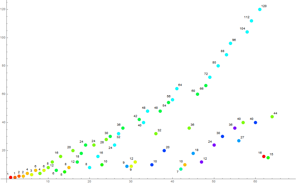
Consider the trajectory of a particular value of τ(m) = t. We increment register ct upon each instance of t as n increases. Certainly t does not always appear as n increases, different values of t occur. However, whenever t occurs, ct increases by 1, thus, we see t ct = m appear in a, furnishing τ(t ct ) → t' ct' . Through this method, we have a trajectory t that occurs with a frequency associated with a range of numbers m that furnish t. These m have a prime power decomposition that supports a given value t. Hence we see certain t grow dominant through a range in n only to be supplanted by a different common t as n increases out of the range.
The differences between records demarcate regimes of preeminence in an imperfect way. We can see that, within the first hundred terms, several t jockey for record-setting status.
1 sets the trivial first record, followed by a(3) = 2 produced by t = 1. Trajectory t = 2 sets a record a(5) = 4, lodging also a(7) = 6. Trajectory t = 4 takes over with a(10) = 8. This trajectory is interrupted by t = 6 with a(19) = 24 only to reclaim record at a(24) = 28, losing out thereafter to t = 6 again with a(25) = 30. Trajectory t = 8 sets its first record a(27) = 32, to be bested by t = 6 with a(28) = 36 and a(32) = 42. Trajectory t = 8 scores a record a(34) = 48, bested by t = 6 at a(39) = 54, in turn bested by t = 8 at a(40) = 56 and a(48) = 64. Trajectory t = 6 sets its last record at a(48) = 66.
Trajectory t = 8 reigns between a(48) and a(87) = 160 inclusive.
Trajectory t = 12 reigns between a(89) = 168 and a(556) = 1380 inclusive.
Trajectory t = 24 reigns between a(558) = 1392 and a(15269) = 58392 inclusive.
Trajectory t = 48 dominates starting with a(15270) = 58416 and is still dominant at n = 220.
Figure 2 is an annotated scatterplot of a(n) for 1 ≤ n ≤ 256. The color function and label pertain to τ(m):
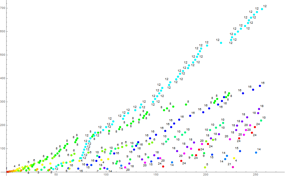
Thus, we see that the cyan-colored trajectory t = 12 increments by 12 at each of appearance of m such that τ(m) = 12. In the pictured range, t = 12 has become dominant.
Figure 3 is a scatterplot of a(n) for 1 ≤ n ≤ 212. The color function pertains to τ(m):
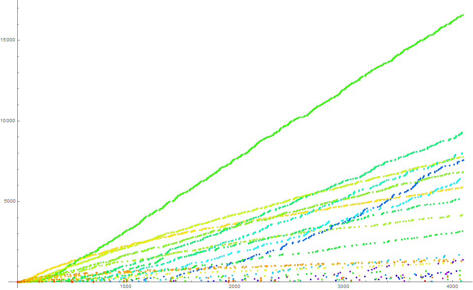
In Figure 3, the cyan trajectory t = 12 is instead colored gold, and is supplanted by t = 24.
Figure 4 is a scatterplot of a(n) for 1 ≤ n ≤ 220. The trajectories t are clearly visible at this scale.
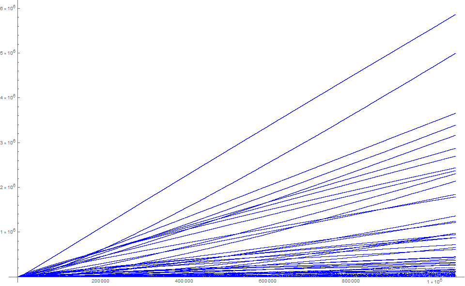
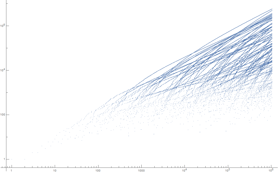
Figure 5 is a log-log scatterplot of a(n) for 1 ≤ n ≤ 220. This scaling function shows the various frequencies that accelerate a given trajectory t, only for the trajectory to abate as n increases. Not every trajectory sets records in a.
 This concludes our examination.
Appendix:
Block[{a = {1}, c},
Do[(If[! IntegerQ[c[#] ], Set[c[#], 1], c[#]++];
AppendTo[a, # c[#] ]) &@ DivisorSigma[0, a[[-1]] ], 2^8]; a]]
Code 2: Generate a(n) (slower algorithm):
Block[{a = {1}, b = {1}},
Do[(AppendTo[a, #]; AppendTo[b, DivisorSigma[0, # ]]) &[
Total@ b[[Position[b, DivisorSigma[0, a[[-1]] ] ][[All, 1]] ]] ], {i, 2^8}]; a]
Concerns OEIS sequences:
A000005: Divisor counting function τ(n).
A343327: a(n).
Document Revision Record.
2021 0323 2245 Draft.
2021 0406 2045 Published.
2021 0412 0730 OEIS number added.