OEIS A340840: Relationship of Highly Composite and Superabundant Numbers.

Written by Michael Thomas De Vlieger, St. Louis, Missouri, 2020 1231.

Abstract.

We examine the relationship between the highly composite and superabundant numbers m using the greatest primorial factor P(ω(m)) and the co-divisor d, recognizing m is a product of primorials. The primitive terms D among the factors d gleaned from the mappings of P(ω(m)) across sequence U that is the union of the highly composite and superabundant numbers serves to admit a compactification of thousands of terms of U. Additionally, the production of a scatterplot (x, y) such that D(x) × P(y) = m gives us insight into the nature of subsequences such as OEIS A166981 and A224078. The primorial factor graph raises interesting questions regarding the “strength” of certain families d and certain tiers k = ω(m), visually evident in the graph. We identify certain “landmarks” in the sequence of highly composite and superabundant numbers related to their intersections as well as those of the superior highly composite and the colossally abundant numbers.

Introduction.

Basics.

This paper concerns itself with the matter of highly composite (HC) and superabundant (SA) numbers.

We begin with the notion of the divisor d | n, that is, n = d × d′, positive integers, listed in row n of OEIS A027750.

We recognize the standard form prime power decomposition of n and the fundamental theorem of arithmetic, which says we may break n down multiplicatively thus:

(1.1) n = p₁^e1 × p₂^e2 × … × p_j^ej × … p_k^ek,

with dissimilar primes p₁ < p₂ < … < p_j < … p_k.

(This is commonly called the “factorization” of the integer n, but we shall refer to it as PD or prime decomposition of n.)

The prime p₁ is the least prime factor lpf(n) = A020639(n) while p_k is the greatest prime factor or gpf(n) = A6530(n). Additionally, we recognize that 1 is the empty product, that is, the product of no primes at all, which is tantamount to the product of any number of primes raised to the zeroth power p⁰ such that mentioning them is pointless. In this work we show a nondivisor prime by q, and recognize that q ⊥ n, i.e., q is coprime to n, meaning the greatest common divisor gcd(q, n) = 1.

The divisor counting function τ(n) = A5(n) represents the number of d | n. The prime divisor counting function Ω(n) = A1222(n) represents the number of primes p | n with multiplicity, while the distinct prime divisor counting function ω(n) = A1221(n) = k addresses only distinct p | n. The former we nickname “big Omega” and the latter “little omega”. Hence, for example, PD(12) = 2² × 3¹ = 2 × 2 × 3, so ω(12) = 2 but Ω(12) = 3, and, via the following formula:

(1.2) τ(n) = Π (e + 1)
for all p^e | n, e > 0,

we see τ(12) = 6, and we can list them via row 12 of A027750: {1, 2, 3, 4, 6, 12}.

The numbers {1, n} are the trivial divisors of n that divide all n, and we observe 1 | n for all n, thus, τ(1) = 1; for n > 1, τ(n) ≥ 2.

The divisor sum function σ(n) = A203(n) is the total of all divisors d | n. Given the prime power decomposition of n, we observe that:

(1.3) σ(n) = Π_{p^e | n} σ(p^e)
with e > 0.

As to prime powers p^e, we have the following formula:

(1.4) σ(p^e) = (p^(e+1) − 1)/(p − 1)

Hence, we generally have:

(1.5) σ(n) = Π_{p^e | n} (p^(e+1) − 1)/(p − 1)
with e > 0.

We may assign a prime p an index i in the sequence of primes A40. Hence, π(p) = i, and we distinguish this usage of π from the circumference-diameter ratio π. Therefore, π(11) = 5, since 11 is the fifth prime, noting 2 is the smallest prime and that it can be demonstrated that there are an infinitude of primes.

The product P(n) = A2110(n) of the n smallest distinct primes p is known as a primorial. The sequence begins:

1, 2, 6, 30, 210, 2310, 30030, 510510, 9699690, 223092870, 6469693230, 200560490130, ...

as 1 is the empty product, 2 is the product of the first prime, 6 the product of the smallest 2 primes, 30 the product of the smallest 3 primes, etc.

Multiplicity Notation.

A method of abbreviating PD(n) is by merely noting the exponents e in the π(p)-th (that is, the i-th) place, writing 0 in the i-th place when q_i ⊥ n. This is tantamount to citing row n of A067255. Hence, for n = 84 = 2² × 3¹ × 7¹, the multiplicity notation or MN(84) = {2, 1, 0, 1}, with 0 in the third place because p₃ = 5 does not divide 84. Here, we write MN(84) thus: 2.1.0.1, since we can have exponents e > 9 and catenation of the exponents to resemble a decimal number eventually proves ambiguous. This is a little-endian flavor of MN that serves a purpose here, though we can also write the exponents in a big-endian way that functions like a number expressed in decimal, with the place i = 1 at left and i = k at right. Technically, we may write an endless number of zeros after the exponent e_k, pertaining to the gpf(n) = p_k, but generally, only write zeros as placeholders when they appear between other numbers in multiplicity notation.

The Highly Composite and Superabundant Numbers.

A highly composite (HC, A2182) number m is such that m sets a record in the divisor counting function sequence A5(n) = τ(n).

The sequence τ(n) begins:

1, 2, 2, 3, 2, 4, 2, 4, 3, 4, 2, 6, 2, 4, 4, 5, 2, 6, 2, 6, 4, 4, 2, 8, 3, 4, 4, 6, 2, 8, 2, 6, 4, 4, 4, 9, 2, 4, 4, 8, 2, 8, 2, 6, 6, 4, 2, 10, 3, 6, 4, 6, 2, 8, 4, 8, 4, 4, 2, 12, ...

Therefore, we see the records {1, 2, 3, 4, 6, 8, 9, 10, 12, …} at indices {1, 2, 4, 6, 12, 24, 36, 48, 60, …}. These are the first terms of A2182 are:

1, 2, 4, 6, 12, 24, 36, 48, 60, 120, 180, 240, 360, 720, 840, 1260, 1680, 2520, 5040, 7560, 10080, 15120, 20160, 25200, 27720, 45360, 50400, 55440, 83160, 110880, 166320, 221760, 277200, ...

The examination of superabundant numbers requires us to disambiguate from the “merely” abundant numbers.

We call n “abundant” if the sum of divisors σ(n) = A203(n) > 2n. We see that 2 × 12 < 28 = 1+2+3+4+6+12, hence it is abundant. The distinction was known to Nicomachus in antiquity.

Superabundant (SA, A4394) numbers m instead relate to the ratio σ(n)/n. Indeed, we deem m superabundant if σ(m)/m > σ(m')/m'for all m' < m. The first numbers in this sequence are:

1, 2, 4, 6, 12, 24, 36, 48, 60, 120, 180, 240, 360, 720, 840, 1260, 1680, 2520, 5040, 10080, 15120, 25200, 27720, 55440, 110880, 166320, 277200, 332640, 554400, 665280, 720720, 1441440, ...

The numbers m, whether HC or SA, are products of primorials, thus A2182 ⊂ A025487 and A4394 ⊂ A025487; the sequence of products of primorials, A025487 itself, is a subset of A055932, which contains numbers that are products of a multiset of the smallest primes p. (At the time of writing, we have drafted A340840 as the union U of A2182 and A4394.)

Therefore, MN(m) in A055932 contains no zeros. Hence, n = 84 is not in A055932 since it is not the product of a contiguous multiset of the smallest primes p, as it has no factor 5, but it does have the factor 7.

Numbers m in A025487 are characterized by nonincreasing multiplicities as i increases. Thus, numbers like 12 and 36 appear in A025487 since MN(12) = 2.1 and MN(36) = 2.2, but 18 is not since MN(18) = 1.2.

Since m in A2182 or A4394 are also in A025487, these numbers share the qualities of the supersets; they are products of a multiset of the smallest k primes p₁…p_k such that their multiplicities e₁ ≥ e₂ ≥ … ≥ e_j ≥ e_k.

The conception of m in A2182 and A4394 as products of primorials has several key consequences:

1. The only odd term is 1.
2. For m > 1, lpf(m) = 2.
3. The only prime m = 2.
4. The only primorial m are {1, 2, 6}.
5. The only square m are {1, 4, 36}.
6. We can identify primorial P(k) | m as the greatest primorial divisor of m, where k = ω(m), hence p_k = gpf(m).
7. There is no nondivisor prime q ⊥ m such that 2 < q < p_k. Therefore, the least q = p_(k+1).

Furthermore, for products m of primorials P(i) = A2110(i), which are in A025487, we can compactify MN so as to have a succinct rendition of a large m. Flammenkamp used a compression for HC in his 124260 and 779674-term datasets that delimited the e using a space-character, and bundled copies of the same multiplicity by writing e and appending a caret followed by the decimal number of repetitions of e. Examples:

HC(120) = 260858031033600, which he compactified to “10 8 3 2^2 1^6”. This unpacks to MN(HC(120)) → 10.8.3.2.2.1.1.1.1.1.1.

HC(120000) has 3450 decimal digits, yet Flammenkamp writes “18 10 7 6 4^3 3^7 2^27 1^947”, which involves 988 terms in the multiplicity notation.

We may express large numbers via a relatively small MN.

In this work, we shall refer to Flammenkamp’s compactification of MN as “tallied multiplicity notation”.

Figure 1.1 shows some multiplicity diagrams of MN(m) for highly composite and superabundant m. The red line of dots represent the greatest primorial divisor g.

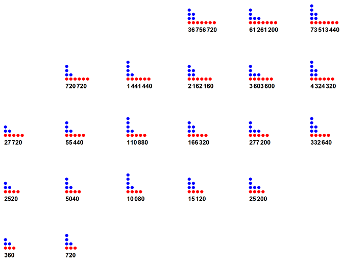
We read the charts by raising the i-th prime p_i to the number e_i of dots in each column i (reading left to right), thus, p_i^e. Therefore n is the product of the p_i^ei. For example, m = 27720 = 2³ × 3² × 5 × 7 × 11, appears at the top of the leftmost column of diagrams. Hence we have a diagram that has columns from right to left that dots as follows: {3, 2, 1, 1, 1}, which is tantamount to MN(27720) → 3.2.1.1.1.

For m in Figure 1.1, ω(m) = the breadth of the diagram as shown by the red dots at the bottom of each diagram, Ω(m) = the number of all the dots in the diagram.

The Conjugate of Prime Power Decomposition.

The definition of A025487 as “products of primorials” is salient, as it grants us insight into another way of representing such numbers. The prime power decomposition of n described above can be seen as reckoning the diagrams in Figure 1 by columns. We can transform these diagrams into a primorial decomposition of n by regarding the rows instead. For example, we have 1, 2, and 5 dots in each row of the diagram pertaining to 27720 = P(1) × P(2) × P(5) = 2 × 6 × 2310.

The expression of highly composite or superabundant m via primorial decomposition is often more efficient for m larger than in the millions.

Example: Flammenkamp[1] noted HC(120000) as “18 10 7 6 4^3 3^7 2^27 1^947”, which involves 988 terms in the multiplicity notation, but its primorial decomposition is 988.41.14.7.4.4.3.2.2.2.1.1.1.1.1.1.1.1. This latter notation might be similarly compressed to “988 41 14 7 4^4 3 2^3 1^8”, which, in terms of characters, is comparable to the Flammenkamp compactification of MN(HC(120000)), i.e. tallied MN.

Representing m as d × P(k).

We are attracted to reckoning m = d × P(k), that is, the product of the greatest primorial divisor P(k) = P(ω(m)) and a number k in A025487 that is the product of all other primorial factors of m. The reason the formulation of m = d × P(ω(m)) is attractive is that it is fairly easy to determine P(k) via ω(m), which serves as an upper bound for all the other primorial factors.

The co-divisor d.

We can derive d easily as well, decoding (MN(m) − 1) and dropping trailing zeros. Thereby, perhaps, we have a handy “family name” via d, since only particular values of d produce m. For example, the HC(25) = 27720 → “3.2.1.1.1” since 27720 = 2³ × 3² × 5 × 7 × 11. Subtracting 1 from each of these values and dropping zeros, but retaining the word length of MN(27720), we have “5: 2.1” → A002110(5) × 2² × 3 = 2310 × 12 = 27720. Indeed it is perhaps easier to merely take

(2.1) d = m / A2110(ω(m)),

which in the case of highly composite m is

(2.2) d = A2182(n)/ A2110(A108602(n)).

and in the case of superabundant m is

(2.3) d = A4394(n)/ A2110(A305025(n)).

It is for this reason that herein, we may refer to any HC number m not as MN(A2182(n)) but as A108602(n): MN(d), both for concision, but also in order to graph such. Similarly, a SA number m can written as MN(A4394(n)) but as A305025(n): MN(d).

Example: A2182(25) = 27720, which we might also know as MN(27720) → 3.2.1.1.1, but we can also write “5: 2.1”. At any rate, the utility of decimal representation for large m or d is perhaps not as high as the multiplicity notation, for from the latter we get an idea of the prime power decomposition of these numbers when very large.

Let’s examine the properties of d. Given that m is a product of primorials, we note the following:

1. The only odd term is 1.
2. The only primorials are {1, 2, 6}, consequently the only square m are {1, 4, 36}.
3. The only perfect powers of 2 (A79) are {1, 2, 4, 8}. These produce m in {1, 2, 6}, {4, 12, 30}, {24, 120, 840}, and {48, 240, 1680}, respectively.
4. Since, by reducing each multiplicity in MN(m) by 1 we derive MN(d), the number d is a product of primorials. Hence d is in A025487.

Families of m.

Let us regard a family of m related to the co-divisor d = m/P(k), and let y = k = ω(m) represent the tier. Alternatively, we may regard the index x of d in the sequence D of primitive d.

Examining the first few highly composite m, we write m = d × P(k) = A301414(x) × A2110(y) at (x, y).

                         x
     |  (1)    (2)    (4)    (6)    (8)    (12)
     |   1      2      3      4      5      6
   ---------------------------------------------
   0 |   1
   1 |   2      4
   2 |   6     12     24     36     48
y  3 |         60    120    180    240    360
   4 |               840   1260   1680   2520
   5 |                                  27720
   ...

(As regards the m shown in the table and the d that appear on the x axis, HC and SA are interchangeable.)

Converting figures in the table to MN and expanding to products m not in A2182 (or A4394):

                         x
     |  (1)    (2)    (4)    (6)    (8)    (12)
     |   1      2      3      4      5      6
   ---------------------------------------------
   0 |   .      1      2      11     3      21
   1 |   1      2      3      21     4      31
   2 |   11     21     31     22     41     32
y  3 |   111    211    311    221    411    321
   4 |   1111   2111   3111   2211   4111   3211
   5 |   11111  21111  31111  22111  41111  32111
   ...

Looking at the multiplicity notation of m in family d, we see that the “tail” of 1s increases in length. Hence each family d includes m whose MN has an incrementally increasing tail.

We see that, for y > ω(D(x)), we see m_(k+1) = m_k × p_(k+1). For x > 1 and for m that are in A340840, y ≥ ω(D(x)). This is to say, generally for m in A340840 holding d constant:

(2.4) m_(k+1) / m_k = p_(k+1)

Highly composite numbers as d × P(k).

Pertinent to HC, given that A2182 strictly increases (since it is a list of recordsetters), we note that i ≤ y ≤ j, integers, for which m = d × P(y) produces HC numbers. As we increment y we increase the rank of the tensor of prime divisor power ranges and double the number of divisors. However, we may have another term m' = a × P(b) for a > d and b < (j + 1) such that m' < m yet τ(m') ≥ τ(m). This m' is in A2182 and has increased tau by the lengthening of the power ranges for relatively small primes via some composite b instead of increasing the rank of the tensor. Since A2182 strictly increases, we have a limited range for m.

(2.5) τ(d × P(y+1)) = 2τ(d × P(y))

Superabundant numbers as d × P(k).

A similar but more complex argument pertains to superabundant m (in A4394). For y ≥ ω(D(x)),

(2.6) σ(d × P(y+1)) = σ(d × P(y)) × (p_(y+1)+ 1)

As we increment y, we multiply σ(m) by (p_y + 1). Thus, σ(m)/m for all m = d × P(y) in family y is rendered by:

(2.7) σ(d × P(ω(d))) × Π_{ j = (ω(d) + 1) …y} (p_j + 1) / (d × Π_{ j = 1…y} (p_j + 1))

Let r = σ(d × P(y−1)) / (d × P(y−1)) and let r' = σ(d × P(y)) / (d × P(y)). Then we have:

(2.8) r' = r × (p_y + 1) / p_y

A4394 strictly increases (since it is a list of recordsetters), we note that i ≤ y ≤ j, integers, for which m = d × P(y) produces SA numbers. So long as there is no other m' = a × P(b) for a > d and b < (j + 1) such that m' < m such that r' < r, we produce SA numbers m with divisor d by incrementing y. Because A4394 strictly increases, constant d produces a limited but continuous range in y of SA numbers m.

Graphing m according to P(k).

Herein we examine the graph of (x, y) such that D(x) × P(y) is m in either A2182 or A4394.

Indeed, we need a sequence D that lists the valid d such that we might use the index x of these valid d in this sequence rather than d itself, which would lead to enormous negative space in any plot, as the d get generally wider apart as d increases.

For the highly composite numbers, we produce a sequence A301413(n) = A2182(n)/A2110(A108602(m)). The sequence begins:

1, 1, 2, 1, 2, 4, 6, 8, 2, 4, 6, 8, 12, 24, 4, 6, 8, 12, 24, 36, 48, 72, 96, 120, 12, 216, 240, 24, 36, 48, 72, 96, 120, 144, 216, 240, 288, 24, 36, 48, 72, 96, 120, 144, 216, 240, 288, 360, 480, 576, 720, 1080, 72, 1440, 120, 144, 216, 240, 288, 360, 480, 576, ...

Thus we take the union of all the terms in this sequence to derive a sequence D_HC = A301414 that contains all the primitive d that produce HC numbers. This sequence begins:

1, 2, 4, 6, 8, 12, 24, 36, 48, 72, 96, 120, 144, 216, 240, 288, 360, 480, 576, 720, 1080, 1440, 2160, 2880, 4320, 5040, 7200, 7560, 8640, 10080, 14400, 15120, 20160, 30240, 40320, 50400, 60480, 90720, 100800, 120960, 151200, 181440, 241920, 302400, 362880, ...

Likewise, for the superabundant numbers, we generate a sequence A305056(n) = A2182(n)/A2110(A305025(m)), which begins:

1, 1, 2, 1, 2, 4, 6, 8, 2, 4, 6, 8, 12, 24, 4, 6, 8, 12, 24, 48, 72, 120, 12, 24, 48, 72, 120, 144, 240, 288, 24, 48, 72, 120, 144, 240, 288, 360, 720, 72, 120, 144, 240, 288, 360, 720, 72, 1440, 2160, 120, 144, 240, 288, 360, 720, 1440, 2160, 2880, 4320, 5040, ...

We take the union of all the terms in this sequence to derive a sequence D_SA = A340014 that contains all the primitive d that produce SA numbers. This sequence begins:

1, 2, 4, 6, 8, 12, 24, 48, 72, 120, 144, 240, 288, 360, 720, 1440, 2160, 2880, 4320, 5040, 8640, 10080, 15120, 20160, 30240, 60480, 120960, 151200, 181440, 241920, 302400, 604800, 907200, 1209600, 1330560, 1663200, 1814400, 3326400, 6652800, 9979200, 13305600, ...

It is clear that certain terms in D_HC are missing from D_SA, for instance, 36, 96, and 216 do not appear in the latter sequence. We also note that there are terms in D_SA are missing from D_HC; the smallest of these is D_SA(116) = 592424239959167616000 which is 12: 9.4.2.1.1. Hence we would require a sequence V = D_SA ∪D_HC in order to represent all m in U = A2182 ∪ A4394.

We note V(315) = D_SA(116). Hence, we can use A301414 to show quite a few m in U so before we miss any superabundant m.

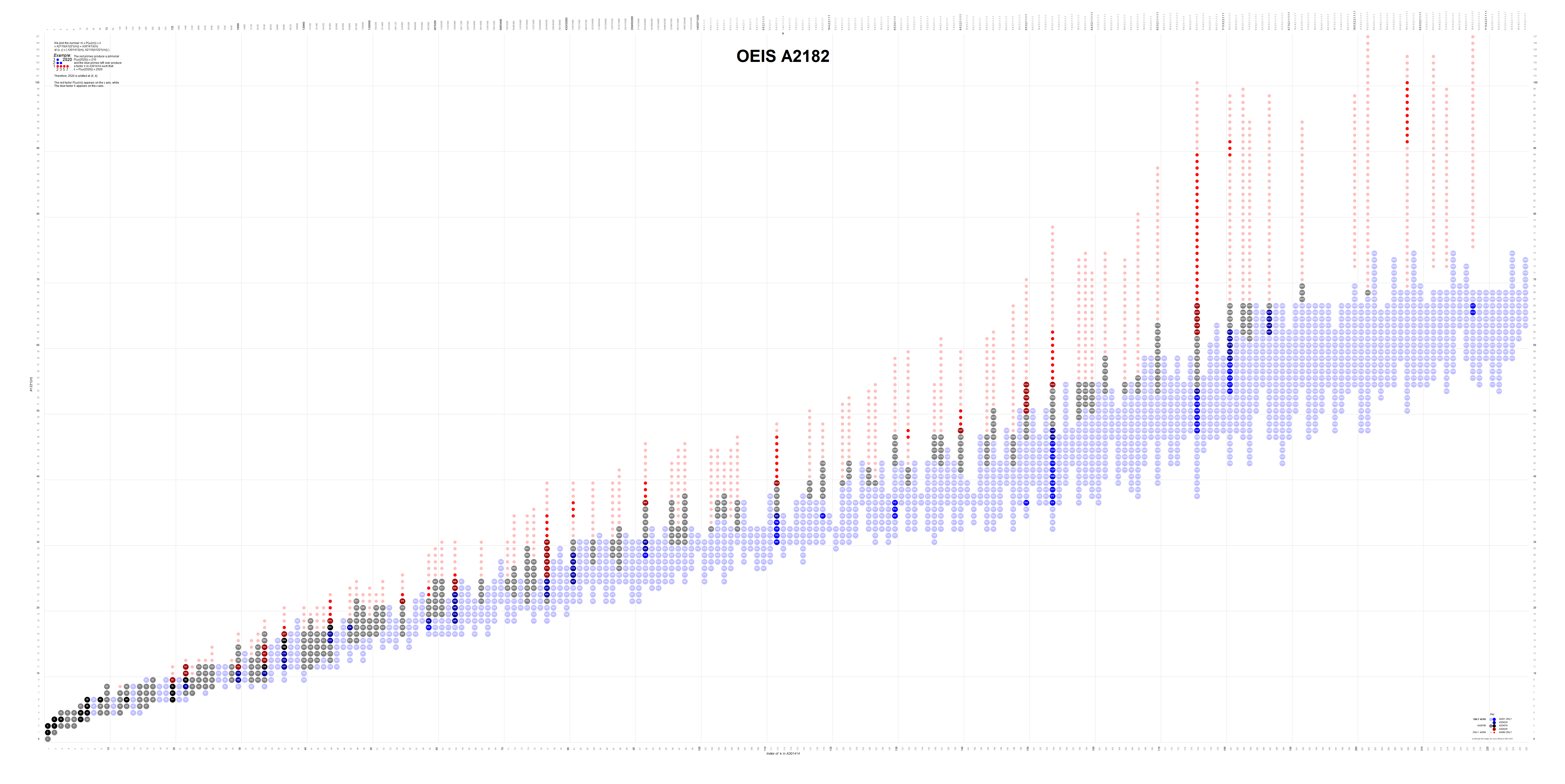
Figure 2.1 is a plot (x, y) such that A301414(x) × A2110(y) is highly composite m in A2182. The products m = A2182(n) are colored blue and assigned their index n.

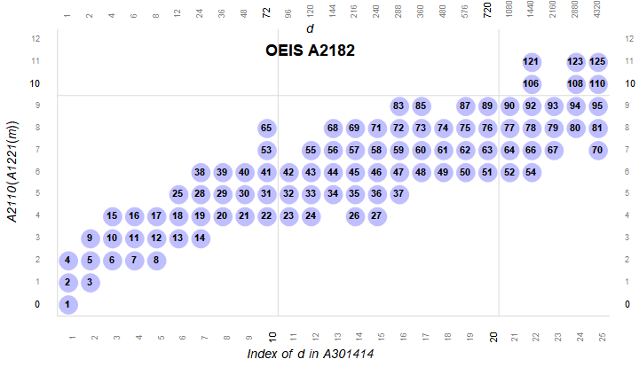
We see demonstrated that we can increment y across a range i ≤ y ≤ j such that d × P(y) = m in A2182. Let d = A301414(x). It is also true that we can increment x and find A301414(x) × P(y) = m in A2182, however, in this axis there are interposing gaps, i.e., P(4), which yields HCs for 3 ≤ x ≤ 12 and 14 ≤ x ≤ 15, but A301414(13) × P(4) = 144 × 210 = 30240 is not in A2182. We see that HC(25) = 27720 has 96 divisors, as does 30240.

Figure 2.2 is a plot (x, y) such that A301414(x) × A2110(y) is highly composite m in A2182. Here we show τ(A2182(n)) = A2183(n), the number of divisors of the HC, in the blue bubble. The figure demonstrates that the number of divisors doubles as y increments as in Equation 2.5.

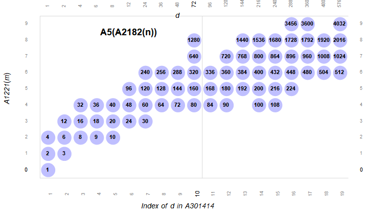
What may strike us is the occasion of perfect powers of 2 in A2183 (as seen in Figure 2.2, the labels in each blue bubble). McRae [5] illustrates through exhaustion that the number of HC numbers that have this property is finite. It seems logical that the other geometric series found among the concatenation of lineages in the columns are likewise finite, since the “prime shape” presented by the diagram of MN(m) at some point will not accommodate the necessary exponents required to support the series. (We have not investigated this.)

Table 2.1 shows the highly composite numbers m such that log₂ τ(m) is an integer:

 i     n    x    y               A2182(n) A2183(n)  MN(A2182(n))
----------------------------------------------------------------
 0     1    1    0                     1        1   0
 1     2    1    1                     2        2   1
 2     4    1    2                     6        4   1.1
 3     6    3    2                    24        8   3.1
 4    10    3    3                   120       16   3.1.1
 5    15    3    4                   840       32   3.1.1.1
 6    20    8    4                  7560       64   3.3.1.1
 7    29    8    5                 83160      128   3.3.1.1.1
 8    39    8    6               1081080      256   3.3.1.1.1.1
 9    50   19    6              17297280      512   7.3.1.1.1.1
10    62   19    7             294053760     1024   7.3.1.1.1.1.1
11    75   19    8            5587021440     2048   7.3.1.1.1.1.1.1
12    87   19    9          128501493120     4096   7.3.1.1.1.1.1.1.1
13   101   31    9         3212537328000     8192   7.3.3.1.1.1.1.1.1
14   116   31   10        93163582512000    16384   7.3.3.1.1.1.1.1.1.1
15   131   31   11      2888071057872000    32768   7.3.3.1.1.1.1.1.1.1.1
16   147   31   12    106858629141264000    65536   7.3.3.1.1.1.1.1.1.1.1.1
17   163   31   13   4381203794791824000   131072   7.3.3.1.1.1.1.1.1.1.1.1.1
...

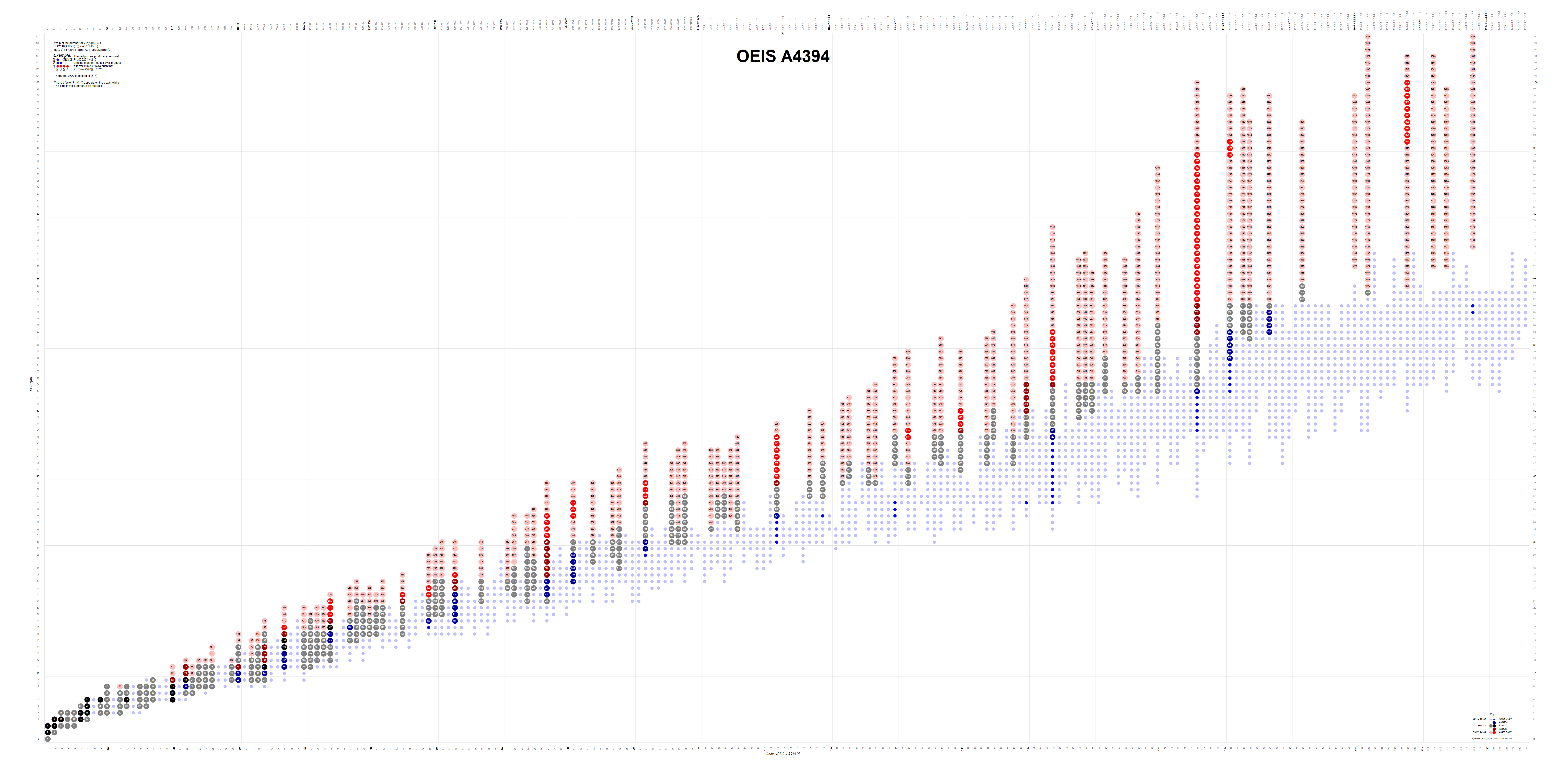
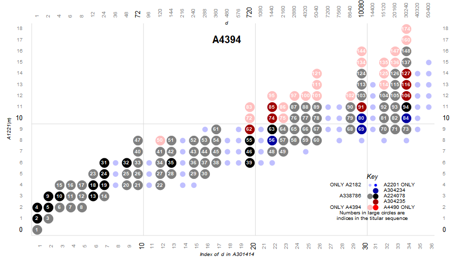
Figure 2.3 is a plot (x, y) such that A301414(x) × A2110(y) is superabundant m in A4394. The products m = A4394(n) are colored pink and assigned their index n.

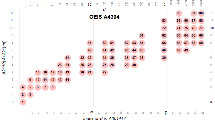
This figure shows that A301414 has terms like 36 and 96, etc. that do not produce SA numbers. Hence we have to use D_SA = A340014 if we are interested in assuredly plotting superabundant numbers.

Figure 2.4 is a plot (x, y) such that A340014(x) × A2110(y) is superabundant m in A4394. The products m = A4394(n) are colored pink and assigned their index n.

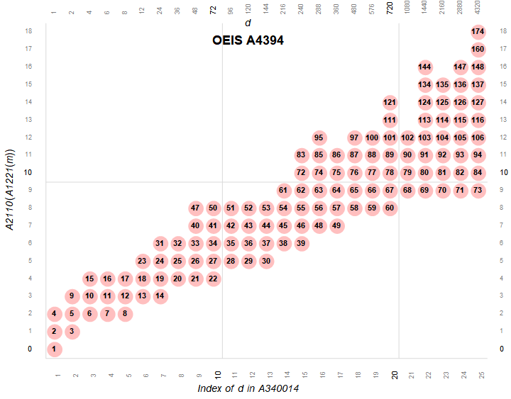
Once again, we can plot m in U = A340840 = union of HCs and SAs and thereby show both using the sequence V = V1250 = union of D_SA and D_HC, however this sequence is tantamount to A301414(n) for n ≤ 314.

Figure 2.5 is a plot (x, y) such that A340014(x) × A2110(y) is superabundant m in A4394. Here we show σ(m)/m in the pink bubble. The figure demonstrates behavior as y increments described by Equation 2.8, namely that for m' = m × p_k where p_(k−1) is gpf of m, σ(m')/m' = σ(m)/m × (p_k + 1)/p_k.

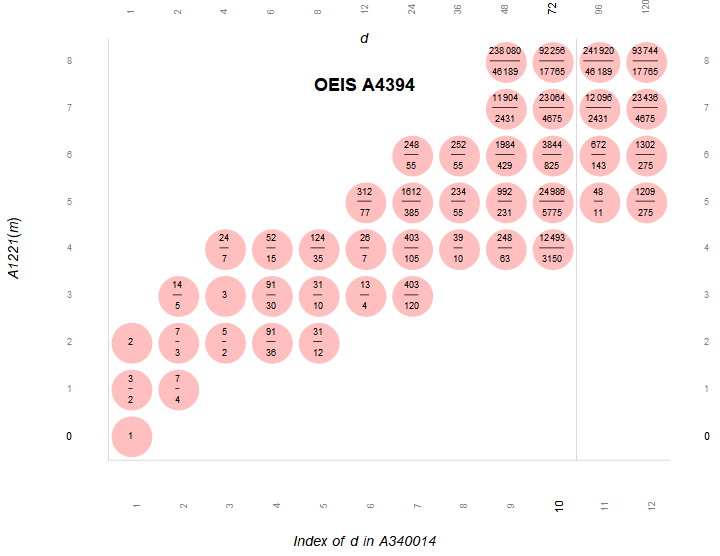
Figure 2.6 is a plot (x, y) such that A340014(x) × A2110(y) is either HC or SA. We know many small HC numbers (blue) are also SA (pink)—these m are in A166981 (gray). The numbers here are indices in a combined HC-SA sequence U(n). (Click for a poster-size map showing all 449 terms m in A166981.)

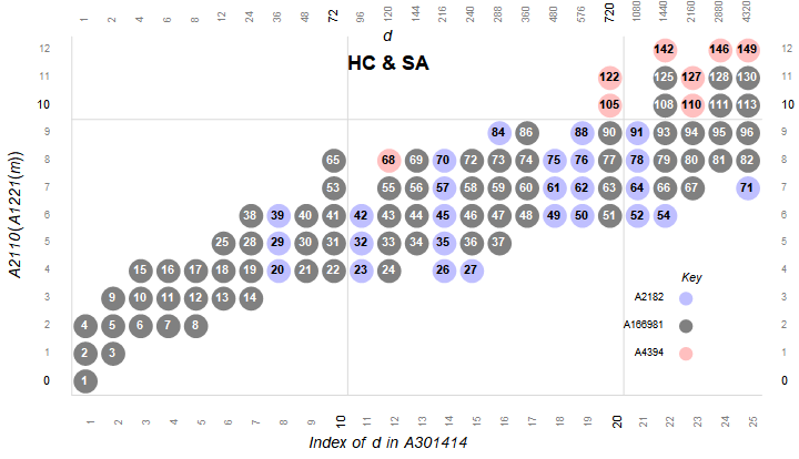
Figure 2.7 is a plot (x, y) akin to Figure 2.5 showing 1 ≤ x ≤ 818 and 1 ≤ y ≤ 442, using V(x) rather than A301414(x):

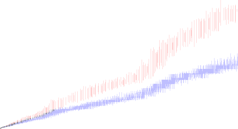
This plot shows all 449 terms of A166981 (see enlarged map) as well as the divergence of A2182 and A4394.

Greatest Primorial Factor Compactification of the HC and SA datasets.

Flammenkamp’s approach to abbreviating MN(m) has been mentioned; we express the multiplicity of exponents using the caret notation, delimiting the terms with a space.

The 3450-digit HC(120000) → “18 10 7 6 4^3 3^7 2^27 1^947” is excellent compression, however, using the conception of m = d × P(k), which for HC is rendered m = A301414(x) × A2110(y), we may simply express it as (2704, 988).

Hence, we may store the entire HC dataset in an image similar to the one below. We read the pixels and find the coordinates (x, y) of black pixels, reconstructing m = A301414(x) × A2110(y).

Figure 3.1 stores 10000 terms m in A2182 at (x, y) → A301414(x) × A2110(y) = m. This image is oriented so as to read as in previous figures, that is, with A2182(1) at the lower left corner. (See an extended plot of Flammenkamp’s 779674 terms.)

The .png image weighs 2,892 bytes, whereas a text file with 4000 terms weighs 518,010 bytes.

Similarly the same thing can be done with SA numbers m = A340014(x) × A2110(y).

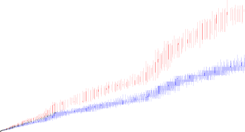
Figure 3.2 stores 10000 terms m in A4394 at (x, y) → A340014(x) × A2110(y) = m. This image is oriented so as to read as in previous figures, that is, with A4394(1) at the lower left corner. (See an extended plot of 100000 terms.)

Remember that the x axes of Figure 3.1 and Figure 3.2 are different and not quite comparable. However, we see that SA numbers tend to have larger greatest primorial factors P(y) for a given D(x) common to the HC numbers.

“Intensifications” of the HC and SA.

The highly composite numbers have an interesting subset Ramanujan named the superior highly composite numbers (SHC, A2201). These SHC are m such that there exists a positive real exponent ε such that:

(3.1)  τ(ℓ)/ℓ^ε ≤ τ(m)/m^ε > τ(n)/n^ε
where ℓ is all numbers less than m,
and where n is all numbers greater than m.

Ramanujan showed the ratio of consecutive SHC terms m is prime; these primes appear in order in A705. Therefore we may produce A2201(n) via the following:

(3.2)  A2201(n) = Π_{i=1..n} A705(i)

The SHC numbers m are products of primorials and are thus in A025487. Thus, we may plot the superabundant numbers as we have the highly composite and superabundant, that is, as a product of the greatest primorial factor P(k) | m and a multiplier d that is also in A025487, such that m = P(k) × d. Taking the union of all d, we arrive at a list D_SHC of primitive d, which is A301416.

The sequence D_SHC = A301416 begins:

1, 2, 4, 6, 8, 12, 24, 36, 48, 72, 96, 120, 144, 216, 240, 288, 360, 480, 576, 720, 1080, 1440, 2160, 2880, 4320, 5040, 7200, 7560, 8640, 10080, 14400, 15120, 20160, ...

Figure 3.3 is a plot (x, y) such that A301416(x) × A2110(y) is superior highly composite. The trajectory is either upward or rightward. Upward moves represent a novel prime q ⊥m as factor of the next term m', while rightward moves represent a prime p | m as an additional factor (with multiplicity) in the next term m'. The numbers in the circles represent the index of m in A2201.

 

Similarly, the superabundant numbers have an interesting subset also studied by Ramanujan and named by him; these are the colossally abundant numbers (CA, A4490).

(3.3)  σ(m)/m^(ε+1) ≥ σ(n)/n^(ε+1)
for all n > 1

The CA numbers are products of primorials and are thus in A025487.

Alaoglu and Erdős proved that the ratio of two consecutive colossally abundant numbers is either a prime or a squarefree semiprime. Hence we may use A073751 to generate A4490 via the following:

(3.4)  A4490(n) = Π_{i=1..n} A73751(i)

The colossally abundant numbers m are products of primorials and are thus in A025487. Thus, we may plot the CA numbers as we have the highly composite and superabundant, that is, as a product of the greatest primorial factor P(k) | m and a multiplier d that is also in A025487, such that m = P(k) × d. Taking the union of all d, we arrive at a list D_CA of primitive d, which is A340137.

The sequence D_CA = A340137 begins:

1, 2, 4, 6, 8, 12, 24, 48, 72, 120, 144, 240, 288, 360, 720, 1440, 2160, 2880, 4320, 5040, 8640, 10080, 15120, 20160, 30240, 60480, 120960, 151200, 181440, 241920, ...

Figure 3.4 is a plot (x, y) such that A340137(x) × A2110(y) is colossally abundant. The trajectory is either upward or rightward. Upward moves represent a novel prime q ⊥m as factor of the next term m', while rightward moves represent a prime p | m as an additional factor (with multiplicity) in the next term m'. The numbers in the circles represent the index of m in A4490.

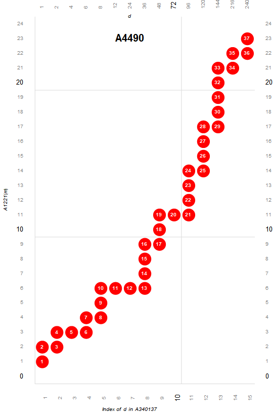
For our purposes, we see the superior highly composite as an intensification of the highly composite, and the colossally abundant as an intensification of the superabundant numbers.

We define sequence V1300 as the union of A2201 and A4490 so as to plot them in the same graph, using the union V1350 of A301416 and A340137 as the font of primitive co-factors d.

The sequence V1350 begins:

1, 2, 4, 6, 8, 12, 24, 36, 48, 72, 96, 120, 144, 216, 240, 288, 360, 480, 576, 720, 1080, 1440, 2160, 2880, 4320, 5040, 7200, 7560, 8640, 10080, 14400, 15120, 20160, 30240, 40320, ...

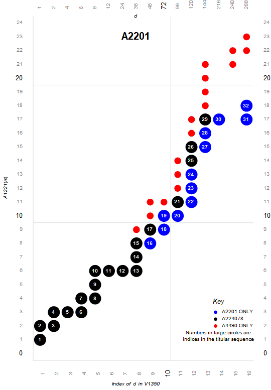
Figure 3.5 is a plot (x, y) such that V1350(x) × A2110(y) is either superior highly composite or colossally abundant (i.e., in V1300). Gaps appear in one or the other trajectory since A301416 is inadequate to show all CA numbers, while A340137 is inadequate to show all SHC numbers quite early in the respective sequences.

Figure 3.5 shows terms m that are both superior highly composite and colossally abundant in black. These 20 terms comprise A224078.

Given the 4 basic sequences we’ve described hitherto, we can plot all using a sequence V(x) = V1250 that is the union of A301414 and A340014, a font of all co-factors d that portray both highly composite and superabundant terms (i.e., their union, A340840).

Figure 3.6 is a plot (x, y) akin to Figure 2.5 showing 1 ≤ x ≤ 818 and 1 ≤ y ≤ 442, using V(x) rather than A301414(x), this time showing the various intersections of A2182, A4394, A2201, and A4490, which will be explained in the next section. (Click for expanded plot showing 151537 terms of A340840, i.e., all m < P(1500).)

Hence, in the primorial factor scatterplot, we enjoy the following relationship:

For m = D(x) × P(y − 1) and m' =D(x) × P(y),
τ(m') = 2 τ(m), and
σ(m')/m' = σ(m)/m × (p_y + 1)/p_y.

Furthermore, we can represent all the various intersections of HC and SA numbers and their intensifications. Given a list of primitive terms d, we may compactify a large dataset of these numbers so as to be reconstructed in a computer algebra system.

For a concordance of the lists of primitive d, this file renders V1250(n) for 1 ≤ n ≤ 1000, relating A301414, A301416, A340014, and A340137.

Flavors of m in A340840.

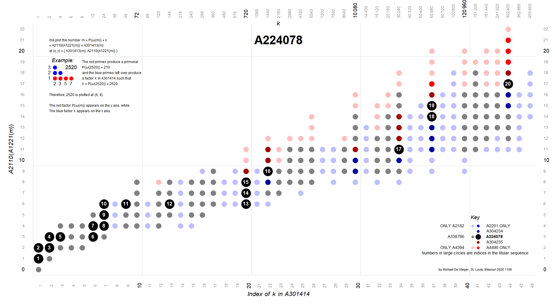
There are 9 possible mutually exclusive subsets or “flavors” of m = V(x) × P(y). These flavors represent regions of terms in the primorial factor scatterplot produced by the intersections of the four sequences A2182 (HC), A2201 (SHC), A4394 (SA), and A4490 (CA).

We assign the highly composite numbers a muted blue and the first bit of a 4 bit number, and the superabundant numbers a muted red and the second bit of a 4 bit number. Since the superior highly composite numbers are a special case of HC, they receive the color blue and the third bit of a 4 bit number, however, if the third bit is on, then so shall be the first bit, thus we cannot have the value 4; we have the value 5. Likewise, the colossally abundant number is a special case of SA, receiving the color red and the last bit of a 4 bit number. Again, since the CA is a special case of SA, when we have the fourth bit on, the second bit is also on, so we cannot have the value 8; instead we have 10. Hence we have the following possibilities:

Table 4.1

4321  dec  seq.    hex color
--------------------------------
0000   0           ffffff  white
0001   1  (A2182)  c0c0ff  light blue
0010   2  (A4394)  ffc0c0  pink
0101   5  (A2201)  0000ff  blue
1010  10  (A4490)  ff0000  red
0011   3  A338786  808080  gray
0111   7  A304234  0000a0  dark blue
1011  11  A304235  a00000  dark red
1111  15  A224078  000000  black

The parenthetical sequences indicate that the code is used to apply to numbers m that are only in said sequence, or in the case of SHC, only also in HC, and CA, only also in SA. The other four flavors have OEIS sequences, and together the four comprise A166981, the intersection of A2182 and A4394. The color key selected is arbitrary and merely used to standardize the plots in this work.

1. Neither HC nor SA.

The first flavor we consider is that m which is neither highly composite nor superabundant. These numbers do not set records in either τ(n) = A5(n) or σ(n)/n = A203(n)/n. In addition to being products m = V(x) × P(y), we include those k in A025487 that do not appear in V, such as perfect powers 2^e for e > 3, and P(j) for j > 2, among other numbers. The reason that V and its subsets A301414 and A340014 exist is to eliminate the invalid terms k in A025487; here we re-introduce them since these make valid numbers in A025487, the superset of the HC and SA numbers. In the plots we’ve shown, this flavor is represented by the white or negative space around the plotted points. In a binary encoding that assigns the identity of the flavor, this flavor appears as 0.

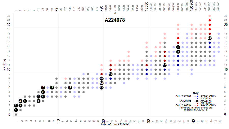
2. A224078: intersection of A2201 and A4490.

The next variety includes numbers that are both superior highly composite and colossally abundant, hence also HC and SA. These m are in A224078, a finite sequence with just 20 terms. These are plotted in black in the following charts and are assigned the color 15. The smallest SHC number not in A224078 (and thus not CA) is 13967553600 = A340840(78) at (22, 8). The smallest CA number not in A224078 (and thus not SHC) is 160626866400 = A340840(90) at (20, 9). The least term in A224078 is 2, while the largest is the 27-digit A340840(275) at (44, 17).

Figure 4.1 highlights the 20 terms m in A224078 (click for an enlarged image with key):

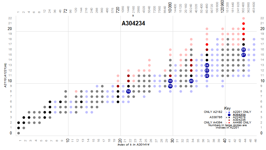
3. A304234: superior highly composite and superabundant but not colossally abundant numbers.

Finite intersection of A2201 and A4394 with 39 terms. The largest term m = A340840(2800) at (187, 65). The smallest SHC that is not in A166981 is A340840(295) at (59, 17). A poster-size map identifying these appears here. Data specific to these numbers appears here. These m are plotted in dark blue and have the binary color code 7.

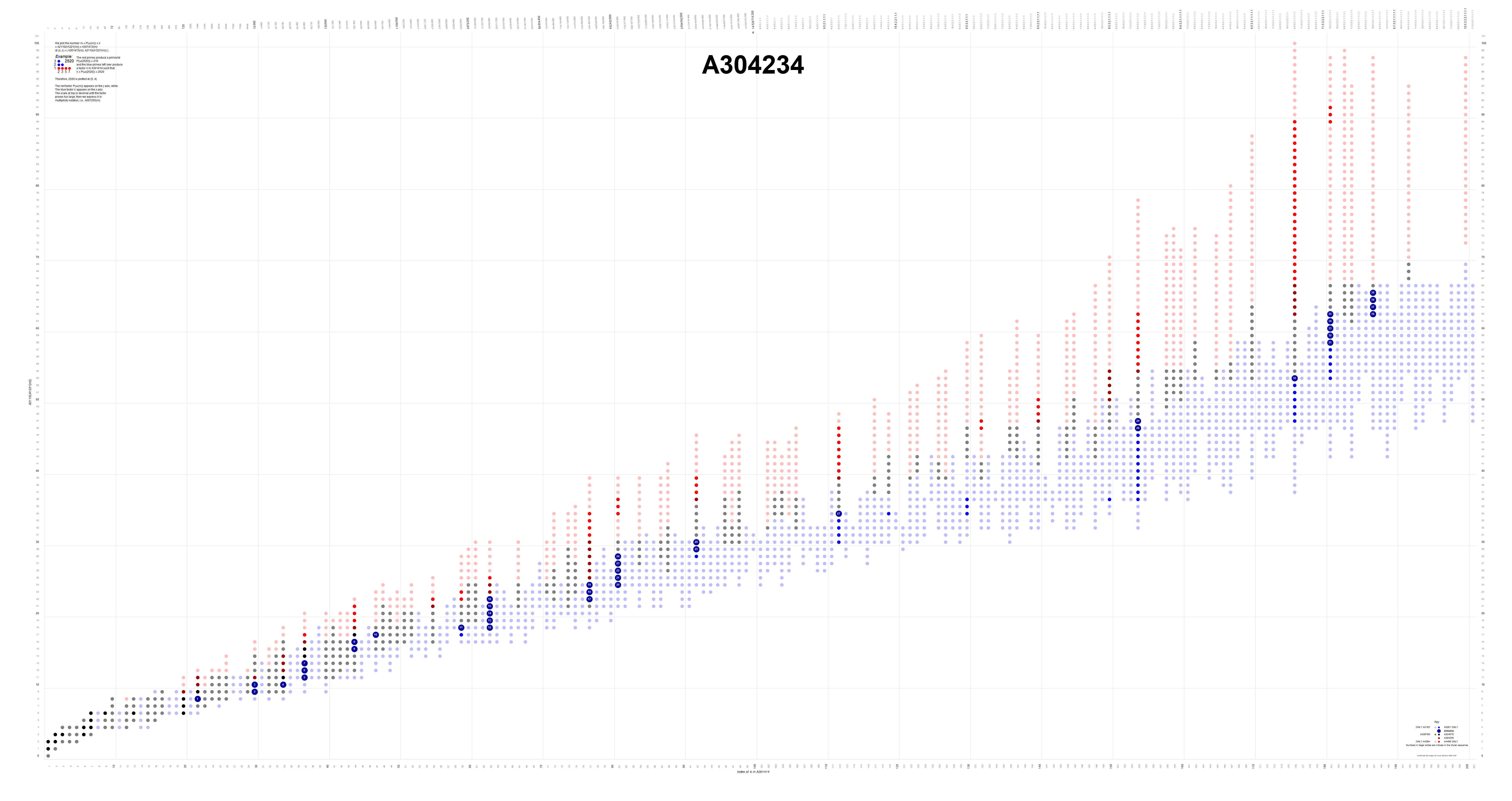
Figure 4.2 highlights the smallest of the 39 terms m in A304234 (click for an enlarged and complete image):

4. A304235: colossally abundant and highly composite but not superior highly composite.

Finite intersection of A4490 and A2182 with 32 terms. The largest term m = A340840(2852) at (176, 66). The smallest CA that is not in A166981 is A340840(263) at (37, 17). A poster-size map identifying these appears here. Data specific to these numbers appears here. These m are plotted in dark red and have the binary color code 11.

Figure 4.3 highlights the smallest of the 32 terms m in A304235 (click for an enlarged and complete image):

5. A338786: numbers in A166981 that are neither superior highly composite nor colossally abundant.

These numbers are both HC and SA but neither SHC nor CA; there are 358 of them. The smallest term is 1. The largest term m is also the largest term of A166981, i.e., A340840(3141) at (192, 69). A poster-size map identifying these appears here. These m are plotted in gray and have the binary color code 3. The m in A338786 can be regarded as numbers in the intersection of A2182 and A4394 that are neither SHC nor CA.

Figure 4.4 highlights the smallest of the 358 terms m in A338786 (click for an enlarged and complete image):

6. A308913*: numbers in A340840 that are only highly composite.

We employ OEIS A308913 as a surrogate for a sequence that would include m that are only highly composite, not SHC or any other flavor. This is an infinite sequence. The smallest term is 7560 = A340840(20) at (8, 4). In the plots in this document, we use light blue (binary color 1) to represent numbers in this rendition of A308913. The smallest term m in A308913 as defined in the OEIS that also appears in A2201 is A308913(269) = A340840(295) at (59, 17). The intent of A308913* is to completely cover all the flavors of highly composite number in the color-coded plots.

Figure 4.5 shows all six regions of A2182. Light blue indicates numbers that are only HC and no other flavor, blue shows numbers that are superior highly composite but not SA, dark blue, numbers in A304234 (SHC numbers that are SA but not colossally abundant). Black indicates numbers in A224078 (that are superior highly composite and colossally abundant). Gray represents numbers in A338786 (numbers that are both HC and SA but neither SHC nor SA), and dark red represents numbers in A304235 (colossally abundant numbers that are also highly composite but not SHC). Together, these comprise the highly composite numbers. Click here for a poster size expansion of this plot with sufficient gamut to show all 449 terms of A166981.

7. A166735*: numbers in A340840 that are only superabundant.

In a similar way to item 5 above, we employ OEIS A166735 as a surrogate for a sequence that would include m that are only superabundant, neither colossally abundant nor any other flavor. This is an infinite sequence. The smallest term is A340840(68) at (12, 8). In the plots in this document, we use pink (binary color 2) to represent numbers in this rendition of A166735. The smallest term m in A166735 as defined in the OEIS that also appears in A4490 is A340840(263) at (37, 17). The intent of A166735* is to completely cover all the flavors of superabundant numbers in the color-coded plots.

Figure 4.6 shows all six regions of A4394. Pink indicates numbers that are only SA and no other flavor, red shows numbers that are colossally abundant but not HC, dark red, numbers in A304235 (CA numbers that are HC but not SHC). Black indicates numbers in A224078 (that are both superior highly composite and colossally abundant). Gray represents numbers in A338786 (numbers that are both HC and SA but neither SHC nor SA), and dark blue represents numbers in A304234 (SHC numbers that are also superabundant but not CA). Together, these comprise the superabundant numbers. Click here for a poster size expansion of this plot with sufficient gamut to show all 449 terms of A166981.

8. A2201*: Superior highly composite numbers that are not superabundant (i.e., not in A304234).

This infinite modified sequence is the set subtraction of A304234 from A002201, which we show as blue. The smallest term in this modified sequence is A2201(31) = A340840(295), plotted at (59, 17).

Figure 4.7 shows 2 of the 3 varieties of superior highly composite numbers. The 20 black terms of A224078 are also colossally abundant. There are 39 dark blue terms in A304234 that are also superabundant but not colossally abundant. An infinite number of blue terms are superior highly composite (and thus also highly composite) but not superabundant. We can see these terms in the poster sized enlargement of A340840.

Figure 4.8 focuses only on the superior highly composite numbers and the colossally abundant numbers. The 20 black terms of A224078 both superior highly composite and colossally abundant. There are 39 dark blue terms in A304234 that are also superabundant but not colossally abundant. An infinite number of blue terms are superior highly composite (and thus also highly composite) but not superabundant. We can see these terms in the poster sized enlargement.

9. A4490*: Superior highly composite numbers that are not superabundant (i.e., not in A304234).

This infinite modified sequence is the set subtraction of A304235 from A004490, which we show as red. The smallest term in this modified sequence is A4490(28) = A340840(263), plotted at (37, 17).

Figure 4.9 shows 2 of the 3 varieties of colossally numbers. The 20 black terms of A224078 are also superior highly composite numbers. There are 32 dark red terms in A304235 that are also superabundant but not colossally abundant. An infinite number of red terms are superior highly composite (and thus also highly composite) but not superabundant. We can see these terms in the poster sized enlargement of A340840.

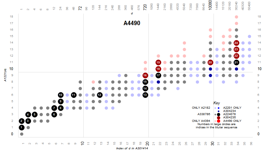
Figure 4.10 focuses only on the colossally abundant numbers and the superior highly composite numbers. The 20 black terms of A224078 both superior highly composite and colossally abundant. There are 32 dark red terms in A304235 that are also superabundant but not colossally abundant. An infinite number of red terms are colossally abundant (and thus also superabundant) but not highly composite. We can see these terms in the poster sized enlargement.

(A166981: intersection of A2182 and A4394.)

The sequences A224078, A304234, A304235, and A338786 comprise A166981, the finite intersection of A2182 and A4394, the numbers m that are both highly composite and superabundant. There are 449 terms in A166981. The least of these numbers is 1 and the greatest is A340840(3141) at (192, 69). A poster-size map of A166981 is here.

Figure 4.11 highlights the smallest of the 449 terms m in A166981 (click for an enlarged and complete image):

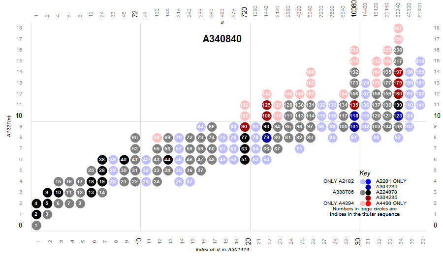
And at long last we can reconstruct the plot of A340840 with all the mutually exclusive flavors shown.

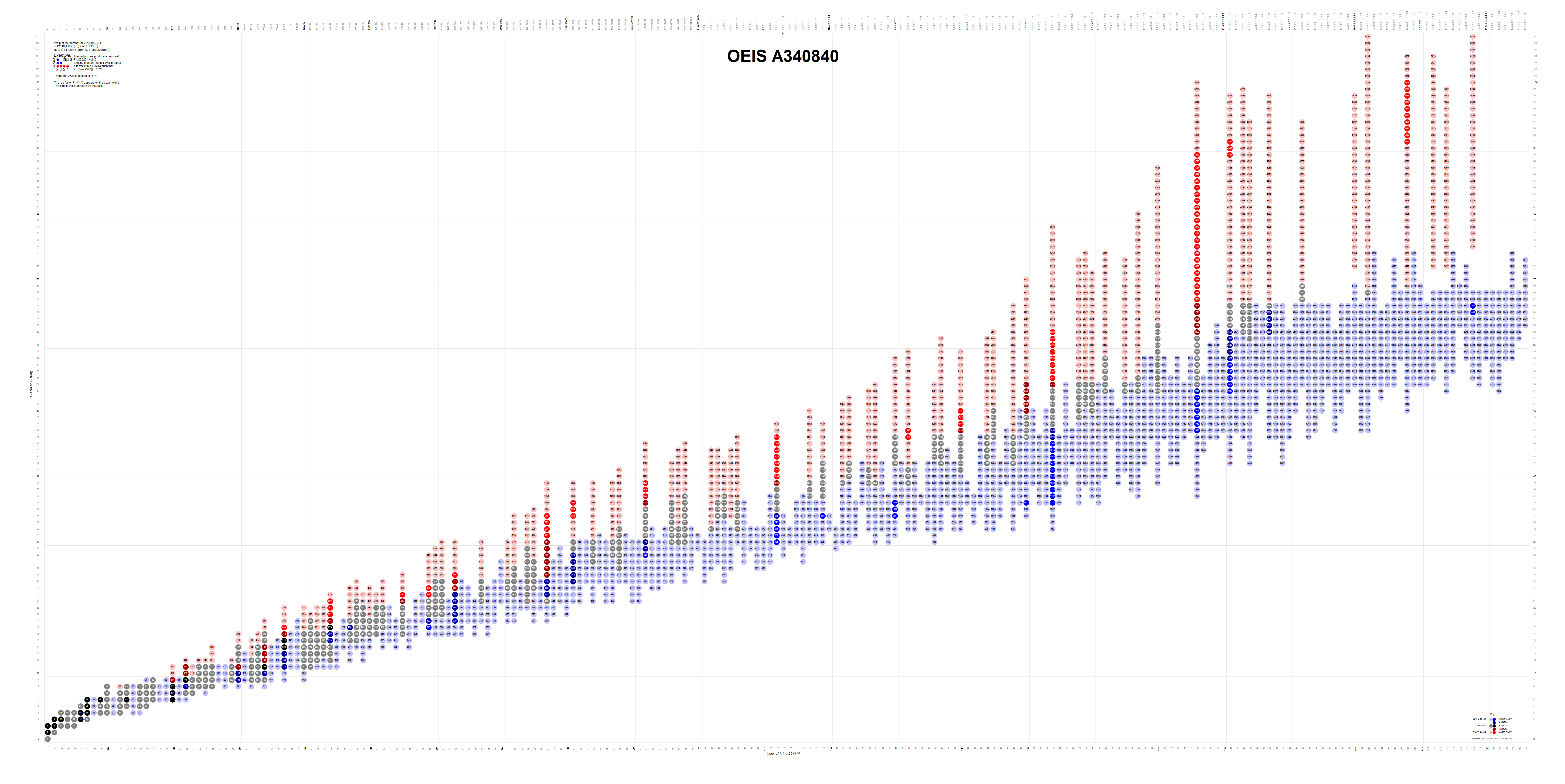
Figure 4.12 maps many of the flavors and assigns their indices in A340840, color coding indicates the flavor per the key. Click for a labeled and annotated poster-sized enlargement sufficient to display all the 449 terms of the intersection of the highly composite and superabundant numbers (A166981), or review the expanded plot showing 151537 terms of A340840, i.e., all m < P(1500). This annotated plot is the original (2018) manifestation of the automated, code-generated plot below.

Landmark terms m in A340840.

In the previous section we mentioned certain points in the scatterplot (x, y) of m in A340840. This annotated poster-sized enlargement of A340840 (as seen in Figure 4.12) relaxes all other points and only labels the terms mentioned in the previous section.

We present here some landmark numbers that represent the least or greatest term of a subsequence or “flavor” of A340840. The landmarks constitute handy references and are gathered here as many are large numbers that are complicated to describe, so as to save space. We will refer to these as terms of A340840.

A340840(1) = 1 = A2182(1) = A4394(1) = A166981(1) , at (1,0).
First number that is both highly composite and superabundant.

A340840(2) = 2 = A2201(1) = A4490(1) = A224078(1) , at (1,1).
First number that is both superior highly composite and colossally abundant.
The only prime HC and SA, the first primorial HC, SA, SHC, and CA.

A340840(3) = 4 at (2,1).
The largest square of a prime that is HC, SA, SHC, and CA.

A340840(4) = 6 at (1,2).
The largest primorial HC, SA, SHC, and CA.

A340840(7) = 36 at (2,1).
The largest square that is HC, SA, SHC, and CA.

A340840(20) = 7560 = A2182(20) = A308913(1) at (8, 4).
MN: 3.3.1.1. (i.e., 4: 2.2).
Smallest highly composite number that is not superabundant.

A340840(68) = 1163962800 = A4394(50) = A166735(1) at (12, 8).
MN: 4.2.2.1.1.1.1.1. (i.e., 8: 3.1.1).
Smallest highly composite number that is not superabundant.

A340840(79) = 13967553600 = A2201(16) = A304234(1), at (22,8).
MN: 6.3.2.1.1.1.1.1. (i.e., 8: 5.2.1).
Smallest term of A304234, smallest SHC not in A224078.

A340840(90) = 160626866400 = A4490(16) = A304235(1), at (20,9).
MN: 5.3.2.1.1.1.1.1.1. (i.e., 9: 4.2.1).
Smallest term of A304235, smallest CA not in A224078.

A340840(263) = 116288545977326780410953600 = A4490(28) = A166735(162) at (37,17).
Tallied MN: 7.4.2^2.1^13. (i.e., 17: 6.3.1.1).
Smallest CA not in A166981.

A340840(275) = 581442729886633902054768000 = A2201(29) = A4490(29), at (44, 17).
Tallied MN: 7.4.3.2.1^13. (i.e., 17: 6.3.2.1).
Largest term of A224078.

A340840(295) = 12791740057505945845204896000 = A2201(31), at (59,17)
Tallied MN: 8.4.3.2^2.1^12 (17: 7.3.2.1.1).
Smallest SHC not in A166981.

A340840(530) = A2201(40) = A304234(19), at (77,24), a 43-digit number.
Tallied MN: 8.5.3.2^3.1^18 (i.e., 24: 7.4.2.1.1.1)
Superior highly composite “tangent” term that appears “almost” colossally abundant in the charts.
Multiply this term by nextprime(gpf) and generate a colossally abundant number.
Largest term with this quality.

A340840(564) = A4490(41) = A304235(13), at (77,25), a 45-digit number.
Tallied MN: 8.5.3.2^3.1^19 (i.e., 25: 7.4.2.1.1.1)
Colossally abundant “tangent” term that appears “almost” superior highly composite in the charts.
Divide this term by gpf and generate a superior highly composite number.
Largest term with this quality.

A340840(2800) = A2201(91) = A304234(39), at (187,65), a 144-digit number.
Tallied MN: 11.7.4.3.2^5.1^56 (i.e., 65: 10.6.3.2.1.1.1.1.1)
Largest term of A304234.

A340840(2852) = A4490(90) = A304235(32), at (176,66), a 144-digit number.
Tallied MN: 10.6.4.3.2^5.1^57 (i.e., 65: 9.5.3.2.1.1.1.1.1)
Largest term of A304235.

A340840(3064) = A166981(448) = A338786(357), at (202,68), a 152-digit number.
Tallied MN: 10.6.4.3.2^6.1^58 (i.e., 68: 9.5.3.2.1.1.1.1.1.1)
Term in A166981 that has the largest d = A301414(202).

A340840(3079) = A2182(2515) at (208,68), a 153-digit number.
Tallied MN: 11.6.4.3.2^6.1^58 (i.e., 68: 10.5.3.2.1.1.1.1.1.1)
Highly composite “tangent” term that appears “almost” superabundant in the charts.
Multiply this term by nextprime(gpf) and generate a superabundant number.
Largest term with this quality.

A340840(3141) = A166981(449) = A338786(358) = A2182(2567) = A4394(1023), at (192,69), a 154-digit number.
Tallied MN: 10.6.4.3^2.2^4.1^60 (i.e., 69: 9.5.3.2.2.1.1.1.1)
Largest term of A166981 and A338786.

Landmarks having to do with the primorial factor scatterplots, with scrutiny, visible for HC numbers here and for SA numbers here:

A340840(3169) = A4394(1028) at (208,69), a 155-digit number.
Tallied MN: 11.6.4.3.2^6.1^59 (i.e., 69: 10.5.3.2.1.1.1.1.1.1)
Superabundant “tangent” term that appears “almost” highly composite in the charts.
Divide this term by its greatest prime divisor and generate a highly composite number.
Largest term with this quality.

A340840(3607) = A4394(1110) at (214,74), a 168-digit number.
Tallied MN: 12.6.4.3.2^6.1^64 (i.e., 74: 11.5.3.2.1.1.1.1.1.1)
Superabundant “tangent” term that appears “almost” highly composite in the charts.
Divide this term by d and multiply by A301414(215) and generate a highly composite number.
Largest term with this quality.

A340840(3609) = A2182(2947) at (215,74), a 168-digit number.
Tallied MN: 12.6.4.3.2^6.1^64 (i.e., 74: 11.7.3.2.1.1.1.1)
Highly composite “tangent” term that appears “almost” superabundant in the charts.
Divide this term by d and multiply by A301414(214) and generate a superabundant number.
Largest term with this quality.

A340840(6297) = A2182(5149) at (420,102), a 251-digit number.
Tallied MN: 14.8.4^2.3.2^8.1^89 (i.e., 102: 13.7.3.3.2.1.1.1.1.1.1.1.1)
Highly composite number such that m at (x + 1, y) is neither HC nor SA.

A340840(46439) = A4394(9691) = at (882,437) = (267s,437), a 1342-digit number.
Tallied MN: 13 9 6 4 3^3 2^14 1^416.
Superabundant number such that m at (x, y ± 1) is neither HC nor SA.
Three terms SA(9661), SA(9692), SA(9721), (268s, 436..438), in conjunction with this term, form a sort of “bottleneck” conspicuous in the large-scale primorial factor plot of A4394.

A340840(181996) = A2182(150249) = (3585,1147) = (3242h,1147), a 4087-digit number.
Tallied MN: 18.11.7.6.5.4^2.3^8.2^30.1^1102.
Smallest “singleton” or “island” HC number such that (x ± 1, y ± 1) is neither HC nor SA.

A340840(246973) = A2182(203317) = (4538,1475) = (4006h,1475), a 5434-digit number.
Tallied MN: 18.12.8.6.5.4^3.3^6.2^41.1^1420.
2nd HC singleton.

A340840(374315) = A2182(313710) = (5608,2064) = (4909h,2064), a 7921-digit number.
Tallied MN: 20.12.8.6.5.4^4.3^9.2^44.1^2002.
3rd HC singleton.

A340840(576025) = A2182(482549) = (7272,2911) = (6259h,2911), a 11639-digit number.
Tallied MN: 20.13.8.7.5^2.4^2.3^11.2^57.1^2835.
4th HC singleton.

A340840(594374) = A2182(497331) = (7226,2980) = (6221h,2980), a 11943-digit number.
Tallied MN: 19.12.8.7.5^2.4^3.3^12.2^53.1^2906.
5th HC singleton.

Conclusion.

This work examined the intersection of the highly composite and superabundant numbers and their related superior highly composite and colossally abundant numbers m as products of their greatest primorial factor P(k) and a co-factor d. We used a list of primitive d to furnish indices x and the index y = k = ω(m) to furnish a scatterplot (x, y) that admits a method of visualizing the terms in various intersectional sequences. These sequences include A166981, the intersection of highly composite and superabundant numbers numbers, and A244078, the intersection of superior highly composite and colossally abundant numbers numbers. This scatterplot, which we named a “primorial factor plot”, has the quality of exhibiting a standard relationship in the vertical axis y, such that for m = D(x) × P(y − 1) and m' =D(x) × P(y), τ(m') = 2 τ(m), and σ(m')/m' = σ(m)/m × (p_y + 1)/p_y. We have explored the various mutually exclusive regions produced by the intersections of the four principal sequences, diagramming them and describing some of their delimiting terms. Finally, we have listed certain landmark terms, indexing them in the union of the highly composite and superabundant numbers, A340840. Further work will examine the nature of the various strengths of the families d for the highly composite and superabundant numbers.

Appendix:

References.

[1]: Achim Flammenkamp, “Highly Composite Numbers”, Downloads appear at the bottom of page and require “gunzip” application.
[2]: D. B. Siano, J. D. Siano, “An Algorithm for Generating Highly Composite Numbers.”, 1994.
[3]: Neil Sloane, The Online Encyclopedia of Integer Sequences. See “Concerns Sequences” for individual links.
[4]: Eric Weisstein’s World of Mathematics, “Highly Composite Number”.
[5]: Graeme McRae, Highly Composite Numbers.

General references:
L. Alaoglu, P. Erdös, On highly composite and similar numbers, Transactions of the American Mathematical Society 56 (1944), pp. 448-469. (Theorem 3 largest prime factor, 4 page 456 two with i = 2 for pⁱ, product of primorials.)
Srinivasa Ramanujan, Highly composite numbers, Ramanujan Journal 1 (1997), p. 119-153.
Michael De Vlieger, On a graph of the divisors (p_ω(m)#, m/p_ω(m)) of highly composite numbers m, (2018), contains Mathematica code.

Concerns OEIS sequences:

The V-series numbers pertain to a list assembled by the author for the study of HC and SA numbers and related topics. These are not intended to supplant the OEIS serial numbers.

A000005: V0011: Divisor counting function τ(n).
A000230: V0051: Divisor sum function σ(n).
A000705: V1400: A2201(n) is product of first n terms of this sequence.
A001221: V0201: ω(n) = Number of distinct prime divisors of n.
A001222: V0202: Ω(n) = Number of prime divisors of n with multiplicity.
A002110: V0111: The primorials.
A002182: V0012: Highly composite numbers (HCNs), i.e., where records are set in A5.
A002183: V0013: Records in A5 = A5(A2182(n)).
A002201: V0014: Superior highly composite numbers (SHCNs).
A004394: V0512: Superabundant numbers: n such that σ(n)/n > σ(m)/m for all m < n.
A004490: V0514: Colossally abundant numbers.
A006530: V1002: Greatest prime factor or gpf(n).
A020639: V1001: Least prime factor or lpf(n).
A025487: V0211: List giving least integer of each prime signature; also products of primorial numbers.
A051903: Maximal exponent in prime factorization of n; greatest term in MN(n).
A055932: V0210: Numbers where all prime divisors are consecutive primes starting at 2.
A067255: V0320: For n = Product_p^e, write e_k in the k-th place, or write 0 if p_k does not divide n.
A073751: V0515: Prime numbers that when multiplied in order yield the sequence of colossally abundant numbers.
A108602: A1221(A2182(n)).
A112779: Largest exponent in the prime factorization of highly composite numbers.
A166735: V1207: Superabundant numbers (A4394) that are not highly composite (A2182).
A166981: V1201: Superabundant numbers (A4394) that are highly composite (A2182).
A168263: Finite intersection of A2182 and A244052 = intersection of A2182 and A060735.
A189228: V1209: Superabundant numbers that are not colossally abundant.
A224078: V1202: Numbers that are superior highly composite and colossally abundant.
A275055: V1020: list of divisors d of n in order of appearance in a matrix of products that arranges the powers of prime divisors p of n along independent axes.
A301413: V1240: Factor d by which A2110(A108602(n)) × d = A2182(n).
A301414: V1241: Primitive values d in A301413 such that d × A2110(m) is in A2182; Numbers d such that d × A2110(m) is highly composite for some m.
A301415: Number of terms m in A2110 such that A301413(k) × A2110(m) is in A2182.
A301416: V1341: Numbers m such that m × A2110(k) is in A2201 for some k.
A304234: V1203: Superior highly composite numbers that are also superabundant but not colossally abundant.
A304235: V1204: Colossally abundant numbers that are also highly composite but not superior highly composite.
A305025: V1231: A1221(A4394(n)).
A305056: V1245: Factor d by which A2110(A305025(n)) × d = A4394(n).
A308913: V1206: Highly composite numbers that are not superabundant (A4394).
A333655: V1208: Highly composite numbers that are not superior highly composite numbers.
A338786: V1205: Numbers in A166981 that are neither superior highly composite nor colossally abundant.
A340014: V1242: Primitive values d in A305056 such that d × A2110(m) is in A4394; Numbers d such that d × A2110(m) is superabundant for some m.
A340137: V1342: Numbers m such that m × A2110(k) is in A4490 for some k.
A340840: V1200: U = Union of A2182 and A4394.
See [3] for these and other A-number sequences in this work.

Other sequences:

These sequences are not in the OEIS but are useful in discussion here:

V1250: V = Union of D_HC = A301414 and D_SA = A340014.
V1350: W = Union of D_SHC = A301416 and D_SA = A340137.

This work is a long time in the making, synthesizing thoughts I have had since age 17, when I stumbled upon a book at Kroch’s & Brentano’s at 29 S. Wabash in Chicago in 1987 to find a book describing the highly composite numbers. The title of the book was The Handbook of Integer Sequences by Dr. Neil Sloane, to whom I am thankful.

I dedicate this work to my wife, Laura. I have named A340840(46439) = A4394(9691) “Laura’s Bridge” in her honor, A340840(3607) = A4394(1110) and A340840(3609) = A2182(2947) “Claire’s Kiss” in honor of my daughter, and A340840(181996) = A2182(150249) “Karl’s Isle” in honor of my son. I am not sure my family shares the joy I have had in thinking about these numbers for 33½ years, but nonetheless, like some stargazer naming a distant feature on a planet or moon in honor of his loved ones, have named the most conspicuous features of the plots to their memory. Love, Michael.

Document Revision Record.

2020 1231 1200 Setup.
2021 0129 2230 Final Draft.