On a graph of the divisors (pω(m)#, m/pω(m)) of highly composite numbers m.
Michael De Vlieger, St. Louis, Missouri, 2018 0328 1030, revised 2018 0428 1700.
Abstract:
Consider the largest primorial that divides highly composite m, pω(m)# = pA108602(m)# and d, the divisor of m such that d = m/pω(m)#. The divisor d takes the k-th value in a sequence a(k), proposed to be A301414(k). This paper is an examination of the graph of the highly composite number (HCN) m as the ordered pair (ω(m), k). We employ Achim Flammenkamp’s smaller dataset of 124260 values of A002182 and have produced a chart wherein all such values appear plotted in a diagram measuring 1011 × 2959 pixels. On this graph, we also show the superior highly composite numbers (SHCNs) in their curious pattern that can be explained by considering A000705. We find the “tiers” A108602(m) that set records for the number of HCNs produced, and the “families” d = a(k) that set records for the number of tiers A108602(m) such that d × A002110(A108602(m)) produces a number m in A002182. Continuing our study, we also examine superabundant and colossally abundant numbers plotted on a similar graph.
Foreword.
In the previous data brief, we examined the intersection of the highly composite numbers A002182 and the highly regular numbers A244052. Comparing the two sequences is interesting because divisors constitute a special case of regular numbers. (A regular integer 1 ≤ r ≤ n divides ne with integer e ≥ 0, while divisor d | ne with 0 ≤ e ≤ 1.) Therefore the question posed is, how many regulars do numbers that set records for the divisor counting function A000005 have? Do they also set records in the regular counting function A010846? The finite intersection of the two sequences contains 13 terms, all of which are in A060735 seen as an irregular triangle T(n, c) = c × A002110(n) with 1 ≤ c < prime(n + 1). These appear in Table 1. In further examining these HCNs in terms of their being products c × A002110(n), releasing the restriction on the value of c, we realize that all HCNs can be charted in terms of this multiple c and A108602(m) for m in A002182, since all HCNs are divisible by some maximum primorial A002110(ω(m)) = A002110(A108602(m)). See Table 2.
Multiplicity Notation.
Achim Flammenkamp [1] produced datasets of the smallest 124,260 HCNs, extended to 779,674 HCNs, that we shall call H. Therein, he annotated the HCNs using what we call in this paper “multiplicity notation”. For n = Product_(pie_i), write ei in the π(p)-th place, starting with the smallest p (little-endian). This is tantamount to A054841(A002182(n)) though this OEIS sequence is big-endian, i.e., written like a decimal number and indeed, it is concatenated. We shall use MN or multiplicity notation, “MN(A002182(n))” to signify this notation.
Looking at MN(A002182(n)), we can see that were we to subtract 1 from all the multiplicities and ignore the trailing zeros, we derive MN(d). We know that A002182(n) has the smallest n primes as distinct prime divisors [4], and additionally the product of primorials (see comments at A002182 at [3]). Thereby, perhaps, we have a handy “family name” for d, since only particular values of d produce HCNs. For example, the 25th HCN, A002182(25) = 27720 → “3.2.1.1.1” since 27720 = 2³ × 3² × 5 × 7 × 11. Subtracting 1 from each of these values and dropping zeros, but retaining the word length of MN(27720), we have “5: 2.1” → A002110(5) × 2² × 3 = 2310 × 12 = 27720. Indeed it is perhaps easier to merely take
(1) d = m / A002110(ω(m)),
which is
(2) d = m / A002110(A108602(m)).
It is for this reason that herein, we can refer to any HCN not as MN(A002182(n)) but as A108602(m): MN(d), both for concision, but also in order to graph such. Example: A002182(25) = 27720, which we might also know as MN(27720) → “3.2.1.1.1”, but we can also write “5: 2.1”. At any rate, the utility of decimal representation for large HCNs or values d is perhaps not as high as the multiplicity notation, for from the latter we get an idea of the prime decomposition of these numbers when very large.
Herein we examine the graph of HCNs m plotted for d = a(k) as (A108602(m), k). (See Graph 3.) Indeed, we need a new sequence that lists the valid d such that we might use the index k of these valid d in this sequence rather than d itself, which would lead to enormous negative space in any plot, as the d get generally wider apart as d increases. We suggest OEIS A301414 as the sequence of d = m / A002110(A108602(m)) for highly composite m (in A002182). On such a graph, we see successive increasing values of n as multiplication of the product P = A002110(A108602(m)) × A301414(k) as multiplication by primes q > prime(A108602(m)) beginning with the next largest q. We see successive increasing values of k as multiplication of P by a larger coefficient that is composite for k > 2.
Properties of Divisor d.
Let’s examine the properties of A301414. Given that highly composite numbers (HCNs) are products of primorials, we note the following:
- The only odd term is 1.
- The only primorials, i.e., terms in A002110, are {1, 2, 6}, consequently the only squares in A002182 are {1, 4, 36}.
- The only terms in A000079 are {1, 2, 4, 8}. These produce {1, 2, 6}, {4, 12, 30}, {24, 120, 840}, and {48, 240, 1680}, in A002182 respectively.
- Since, by reducing each multiplicity in MN(m) by 1 we derive MN(d), the number d is a product of primorials. We have merely divided m by its largest primorial divisor. Consequently, A301414 is a subset of A025487, which is a subset of A055932. This means to say that d is a product of a contiguous set of smallest primes wherein the multiplicities do not increase as the prime divisor increases. (This chart shows positions in A301414 of numbers in A055932 and other sequences).
Also given that A002182 strictly increases, we note that i ≤ m ≤ j, integers, for which P = k × A002110(m) produces HCNs. As we increment m we increase the rank of the tensor of prime divisor power ranges and double the number of divisors. However, we may have another term P' = a × A002110(b) for a > k and b < (j + 1) such that P' < P yet τ(P') ≥ τ(P). This P' is in A002182 and has increased tau by the lengthening of the power ranges for relatively small primes via some composite b instead of increasing the rank of the tensor. Since A002182 strictly increases, we have a limited range for m.
The H dataset generates a graph that measures n × k = 1011 × 2959 pixels. (See Graph 4.) To ensure we have indeed found true terms for A301414, we only consider the smallest 2500 terms, rather than 2959. Much greater than 2500, there might be divisors d not in A301414, since we have not yet considered primorials A002110(n) such that d × A002110(n) appears in A002182; these would be larger than those in H. We also have not observed A301415(k) for k much greater than 2500, though the extension of that data is not difficult; the products m associated with these extensions would also exceed the largest term of H. Consider the primorial Q = A002110(1011), a 3436 decimal digit number larger than both A002182(119324) and A002110(1011) × A301414(985). Since A002182 strictly increases and since all highly composite terms m < Q are known and exist in H, we have confirmed at least 2500 terms in A301414.
(On 24 April 2018, the 779,674 values in H were processed, confirming 8000 terms of A301414 in a similar manner. See the extended Graph 4, which is too large to show on a web page.)
The largest m that is the product of a primorial and some A301414(k) with k ≤ 2500 is A002182(112986) → 952: 15.10.6.5.3.3.2.2.2.2.2.2.2.1.1.1.1.1.1.1.1.1.1.1.1.1.1.1.1.1.1.1.1.1.1.1.1.1.1.1, a 3305-digit decimal number with k = 2499. The largest m that is product of some primorial and A301414(2500) is A002182(106405) → 915: 17.10.6.5.4.3.2.2.2.2.2.2.1.1.1.1.1.1.1.1.1.1.1.1.1.1.1.1.1.1.1.1.1.1.1.1.1.1.1.1, a 3162-digit decimal number. Some of the smallest terms of A301414 are explored in Table 5.
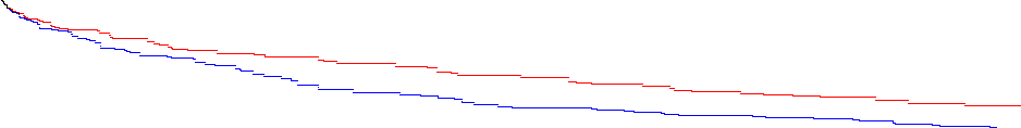
In having produced graphs of the HCN in Flammenkamp’s smaller dataset of 124260 HCNs [1], we note a strong directionality. The k-axis is longer than n = A108602(m), so we might “flop” the chart for reasons of space on the page. We also note the record-setting extents of parameters of these graphs, such as the record-setting number of colored pixels for a given n and k, in Table 6 and Table 7.
General Observations.
We note the curious way the terms in A002201 (Ramanujan’s superior highly composite numbers or SHCNs), a subset of A002182, appear for certain k on the graph. SHCNs appear for certain k, and when it exhausts the n for which A002110(n) × a(k) is in A002182, the value of n is preserved but k jumps to a higher value. This leads to graphing m in A002201 in much the same way to get a “zig-zag” sort of line graph that involves only rook-like vertical or horizontal moves. This is explained in Observation 4.4 and in Graph 8.
In analyzing the ω(d) for d in A301414, we see a general increase in the sequence (see Observation 4.1). Analysis of A051903(d), the largest multiplicity of a prime divisor in d, which in all cases must pertain to the prime 2, shows a general increase but with a lot more dithering than ω(d). These analyses aimed toward attempting to explain the “shagginess” or variation in the vertical “breadth” at column k (i.e., A301415(k)) in Graph 4. These analyses do not seem to explain the variation of terms in A301415.
Graphing Both Highly Composite and Superabundant Numbers.
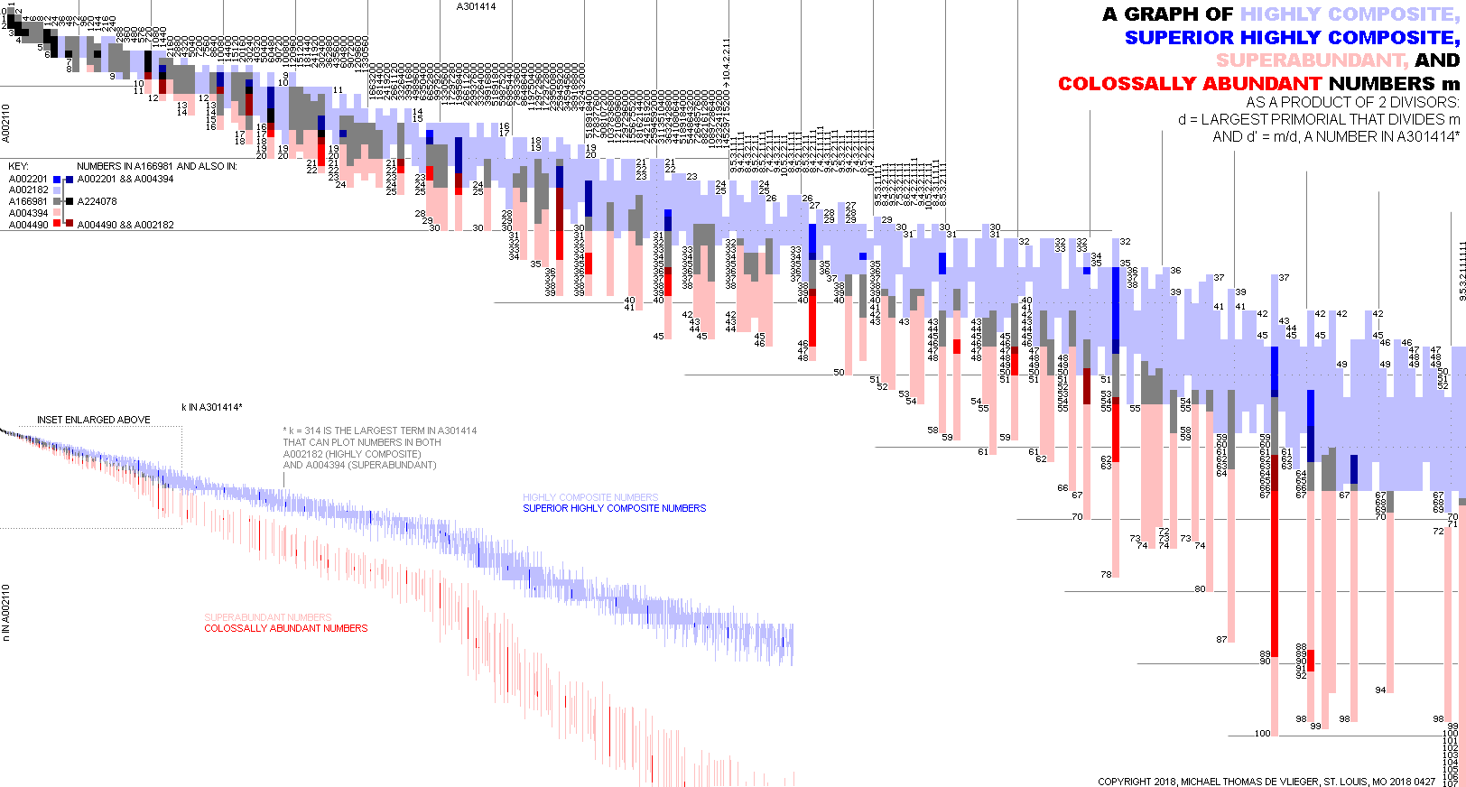
It would seem interesting to chart HCNs and the superabundant numbers (i.e., m in A004394). Graph 9 plots the HCNs in blue and the superabundant numbers in red, with the 449 terms in the finite sequence A166981 in black, i.e., those numbers that are both highly composite and superabundant. The graph shows the “divergence” of the superabundant and highly composite numbers, with the former generally the product of a larger primorial and smaller divisor d. The graph makes evident the fact that A301414 is not sufficient to represent the divisors d of superabundant m = A002110(ω(m)) × d, and that a sequence b(k), like A301414(k) that registers the d with regard to superabundant m would have 314 smallest d in common with A301414, then additional terms. It is not known whether A301414(k) and b(k) eventually become fully distinct as k increases.
Let’s go further, and indicate several classes of numbers shown in Graph 9. In Graph 10, we relax the blue of HCNs and the red of superabundant numbers; where an ordered pair pertains to both, we show gray. In Graph 10 we find there are SHCNs that are also superabundant (dark blue) and colossally abundant numbers that are also highly composite (dark red), as well as ordered pairs that are both superior highly composite and colossally abundant (black). The 20 black pixels correspond to terms in the finite sequence A224078. We might only show the SHCNs and colossally abundant numbers in blue and red respectively on their own charts (Graphs 10.2 and 10.3) and note how these two sequences diverge.
Graph 10.1 seems to be a nice way to visualize and summarize the aggregate properties of the highly composite and superabundant numbers, as well as the superior highly composite and colossally abundant numbers.
We propose the following sequences related to this paper:
A301413: a(n) = A002182(n)/A002110(A108602(n)). Data: 104 terms; Mathematica code. (A dataset of 124260 terms exists.)
A301414: Values d in A301413 such that d × A002110(m) is in A002182; Numbers d such that d × A002110(m) is highly composite for some m. Data: 8000 terms; Mathematica code. Essentially union of 779674 terms of A301413, eliminating the latter terms where it is evident not all information is available to ensure the terms are in order.
A301415: Number of terms m in A002110 such that A301413(k) × A002110(m) is in A002182. Data: 8000 terms; Mathematica code. (pending).
A301416: Numbers m such that m × A002110(k) is in A002201 for some k. Data: 170 terms; Mathematica code. (pending A301415).
Tables and Charts.
Table 1: The intersection of A002182 and A244052.
Table 2: Plot {A108602(m), m/A002110(A108602(m))} for m in A002182..
Graph 3: (A108602(m), k) for m in A002182 and d in A301414(k).
Graph 4: Expand Graph 3 to full dataset of 124260 HCNs.
Table 5: A301414: m/A002110(A108602(m)) for m in A002182.
Table 6: Families k that set records for “breadth” or number of tiers n such that A002110(n) × A301414(k) is in A002182.
Table 7: Tiers A002110(n) that set records for number of values A301414(k) such that A002110(n) × A301414(k) is in A002182.
Graph 8: Plot SHCNs at (A002110(n), A301416(k)) where index n pertains to A002110 and index k pertains to A301416.
Graph 9: Plot HCNs and Superabundant Numbers.
Graph 10: Superior Highly Composite and Colosally Abundant Numbers.
(Observations and conjectures follow each table.)
Code.
Table 1: The intersection of A002182 and A244052.
This table originally appears as part of the data brief for A301892. It is from the realization of the intersection of these two sequences that the notion of plotting this graph developed.
The intersection of A002182 and A244052 is finite, consisting of 13 terms:
{1, 2, 4, 6, 12, 24, 60, 120, 180, 840, 1260, 1680, 27720}.
All of these terms are also in A060735 and not in A288813, as the latter are squarefree and have “gaps” among prime divisors. This intersection has the following number of terms in the “tiers” 0 through 5 of A244052:
{1, 2, 3, 3, 3, 1}.
Let a “tier” n consist of all terms m in A244052 with A002110(n) ≤ m < A002110(n + 1). If we look at A060735 as a number triangle T(n,k) = k × A002110(n) with 1 ≤ k < prime(n + 1), the terms are:
{0, 1},
{{1,1}, {1,2}},
{{2,1}, {2,2}, {2,4}},
{{3,2}, {3,4}, {3,6}},
{{4,4}, {4,6}, {4,8}},
{5,12}
The terms are plotted below. The top figure is the ordered pair (n, c) such that A002110(n) × c is in A060735. The middle figure is the decimal number, and the bottom set of numbers delimited by “.” are the exponents of the prime pertaining to the place in which the exponent appears. For example, “2.1.1” → 2² × 3 × 5 = 60.
Observations
- The terms in the multiplicity notations of these numbers hold or decrease. For c = 3 or c = 5, we would have 1.2, 1.2.1, 1.2.1.1, or 1.1.2, 1.1.2.1, 1.1.2.1.1, etc. Such configurations of prime divisors are absent from terms in A002182. Since HCNs are products of primorials and since they have nondecreasing multiplicities of prime divisors that are a contiguous set of the smallest primes, the intersection of A002182 and A060735 must be finite, and only for those c that have nondecreasing multiplicities of prime divisors that are also a contiguous set of the smallest primes.
- The number c = d = 1 is the only odd value in A301414 as it is the empty product, and since d, like the HCN themselves, must be the product of a contiguous set of the smallest primes with multiplicities that are nondecreasing. As such, we know that the HCNs produced by d = 1 are also finite; the only primorials pi# in A002182 are {1, 2, 6}; τ(pi#) = 2i, and we know that since 2 is the smallest prime, for primorials pi# greater than p2# = 6, we can always produce a smaller number with (i − 1) distinct prime divisors that, through the multiplicity of the smaller prime divisors, has more divisors than the primorial pi#. For p3# = 30 with 8 divisors, we have 24 = 2³ × 3 with as many. For p4# = 210 with 16 divisors, the number 120 = 2³ × 3 × 5 has as many.
- If we were to extend the irregular triangle beyond c < p(n + 1), then we could perhaps plot all terms of A002182 on a grid. In the grid below, dots “.” appear for terms in A060735, if not occupied by a term in A002182, which if in A060735 is followed by an asterisk. These dotted and asterisked positions are fully occupied by many but not all terms in A244052 and illustrates some of the “divergence” of the two record-setter sequences.
- Since we observe the terms plotted on a grid tend to occupy certain values of d, we might condense the grid and merely annotate coordinates for each of the terms. We can use
{ω(m), m/A002110(ω(m))} = {A108602(i), A002182(i) / A002110(A108602(i))} to furnish T(n, k).
Table 2: Plot {A108602(m), m/A002110(A108602(m))} for m in A002182.
This is a condensed table similar to that of Observations 1.2 and 1.3. The ordered pair {n, d} may have d further abbreviated to multiplicity notation, but are presented decimally here.
Observations
- The d-values appear to occupy “streets” of certain values:
{1, 2, 4, 6, 8, 12, 24, 36, 48, 72, 96, 120, 144, 216, 240, 288, 360, 480, 576, 720, 1080, 1440, 2160, 2880, ...} = A301414. - The chart resembles the periodic table, except that the range of valid values evacuate the smaller d-values as n increases. Some interposing d-values appear for (n + 1) while other d-values valid for (n − 1) prove invalid in column n, even though they are flanked above and below by valid d-values.
- d = 72 is curiously “strong”, valid for 4 ≤ n ≤ 8. This seems true also for d = 1440.
- Terms in A002201 seem to appear in clusters:
{1,1}, {2,1}, {2,2}, {3,2}, {3,4}, {3,12}, {4,12}, {4,24}, {5,24}, {6,24}, {6,48}, {6,144}, {6,720}, {7,720}, {8,720}, {9,1440}, ...
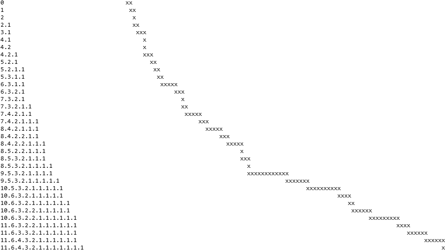
Graph 3: (A108602(m), k) for m in A002182 and d in A301414(k).
What do these numbers look like plotted on a graph with n = number of distinct prime divisors and k an index of the primitive values of d?
Mathematica output involving the smallest 10,000 HCNs obtained at [1].
We place an “x” at the location of an HCN according to the ordered pair{n, d}, with tier n = A108602(m) horizontally starting with n = 0, and where here we speak of k as the index of m/A002110(A108602(m)) in A301414, shown vertically, starting with 1 The first figure at right of each row is A301414(k), and the last figure is MN(A108602(m)).
We place an “0” at the location of a SHCN (m also in A002201).
This is a compressed version of Tables 3 and 4, an abridgement of the data available in the b-file at A002182.
Observations
- Though there may be gaps vertically, the rows seem to be solid. This is observed for the smallest 2600 values of k. This seems to imply the following. Given pω(m)#, and k, the smallest number whose product P = k × pω(m)# is in A002182, we can multiply P by successive primes greater than pω(m) and perhaps produce more HCNs. Once we produce P not in A002182, that family k is exhausted.
- Below we show the order of generation of the chart, plotting m (mod 10) at (n, k) with n = ω(m), so as to continue to show the HCNs with a single character. Generally, the HCNs appear in vertical runs, sometimes and increasingly interrupted by m at higher values of n. In order of appearance, we have highly composite 1 (here presented decimally) at (0, 1), then 2 at (1, 1), 4 at (1, 2), (cf. Table 2). The first occasion wherein we see a number m appear in column (n + 1) while column n is not yet exhausted is 27720 at (5, 6) appearing before 43560 at (4, 14). :
- Interesting “strong” families (here, MN(d)) such as 3.2, 5.2.1, 5.2.1.1, 5.3.1.1.1, etc.
- Interesting “choke points” at 9: 4.3.1, n = {29, 30} family 10.4.2.2.1.1, and more severely, 32: 10.4.2.2.1.1.1 and 36: 8.6.2.2.1.1.1.
- The “energy” seems to transfer around 18: 6.4.2.2 such that for n < 18 the HCNs are mostly and solidly in families d < 6.4.2.2 → 6350400, but for n > 18, the HCNs are mostly and solidly in families d > 6350400.
- In using the first 216 terms of Achim Flammenkamp’s “HCN_NO” data, an expanded chart reveals
an actual “disjunction” between families 14.9.4.4.2.2.2.2.1.1.1.1.1.1.1.1.1.1.1.1 and 14.8.4.3.2.2.2.2.2.1.1.1.1.1.1.1.1.1.1.1, where the former does not produce HCNs for 5 tiers until the latter begins to produce HCNs. - The “amplitude” of the families (meaning the start and end of row k) seems to increase and dominate over tiers as k increases.
- Superior highly composite numbers appear in “rows” at particular families, for example, the five SHCNs at tiers 11 ≤ n ≤ 15 inclusive at family 6.3.1.1. (i.e., the 22nd through 25th terms in A002201, specifically, 12129898443062400, 448806242393308800, 18401055938125660800, 791245405339403414400, 37188534050951960476800).
- In examining a larger dataset, we note that a given k may produce consecutive SHCNs for n, but then jump to a larger k to produce an SHCN in the same n, much like the motion of a rook. This implies we might chart these as well.
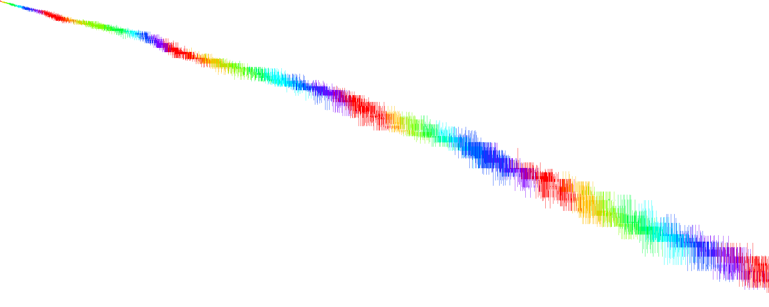
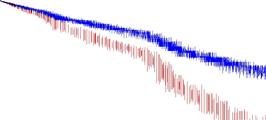
Graph 4: Expand Graph 3 to full dataset of 124260 HCNs.
Let’s dispense with text and attempt to plot as many HCNs as possible.
If we take the investigation quite far, we produce the following plot of 124620 terms provided by [1]. The black pixels represent a HCN (i.e., m in A002182) while the red pixels represent a SHCN (i.e., m in A002201, also in A002182, since A002201 is a subset of A002182). The HCNs plotted here derive from [1], while the SHCNs plotted in red derive from my processing the 104 term b-file at A000705.
The 779,674 terms available in the larger dataset H was processed, furnishing an extended graph that measures 8563 × 4096 pixels. This graph is too large to show on most screens in a web page, but it can be viewed as a graphic.
Observations.
- We must bear in mind that the families k do not represent a scalar, but instead select values of d that are in order of numeric magnitude, but not in necessarily in an order according to prime decomposition. For instance, the first values are {1, 2, 4, 6, 8, 12, 24, 36, …}, which have MN {0, 1, 2, 1.1, 3, 2.1, 3.1, 2.2, …}.
- There are certain families that produce HCNs across a range of tiers n, while there are others that are disjunct from tiers in the previous or next family. For instance, the 16th record for vertical length (30 tiers) is k = 176, a(k) = 809559406656000, with MN 9.5.3.2.1.1.1.1.1.
- There are ranges of consecutive families that generally produce HCNs at more or less the same range of tiers. An example occurs between (n, k) = (138, 509) and (153, 547); a(153) = 387781144204626083601930240000 and a(547) = 85232014430622668316388961280000.
- The red pixels correspond to SHCNs, terms m in A002201. We recall that A002201(i) is the product of the first i terms in A000705, where in all terms are prime. It follows that the red pixels, starting at (1,1), either “advance downward” (n increases) or “advance rightward” (a(k) has a different prime decomposition while A301414(j) increases in magnitude). The “downward” move results in producing consecutive terms in A002201 because these are cases where A000705(i + 1) introduces a new prime q not already in the sequence. The jumping right of the red pixels represents those cases wherein A000705(i + 1) is a prime p already in that sequence.
- The graph confirms all k < 2661 and n < 1005.
- Note: On 24 April 2018, the 779674-term dataset at [1] allows us to extend the graph to confirm all k < 8112 and n < 4090.
- The extension reveals the overall trajectory of the data proceeds more “southeasterly” than the “east-southeasterly” direction that the graph featured here shows. The turning point occurs around (1100, 3250).
- The extended graph shows an interesting seeming “braid” structure around (2900, 6250), where the path of pixels weaves between two dense blocks.
The divisor A301414(k) produces HCNs only in a narrow but continuous range of n that has length A301415(k). Since its range is continuous, we can denote the minimum and maximum values of n for which A002110(n) × A301414(k) is in A002182. We can also see if ω(A301414(k)) or the maximum multiplicity of A301414(k) (i.e., A051903(A301414(k)) ) generates the “shagginess” or variation in A301415(k) for k in a given small range.
Let’s look at the range 40 ≤ n ≤ 100 and 190 ≤ k ≤ 310 (i.e., coordinates (40, 190) to (100, 310) in Graph 4.
The image on the right shows the area in question. The center image shows columns k with ω(A301414(k)) = 8 generally at left in purple, 9 generally in the center in red, and 10 generally at right in green. The right image shows columns k with A051903(A301414(k)) = 8 in red at left, 9 in yellow throughout, 10 in green throughout, 11 in cyan throughout, and 12 in dark blue trending to the right. These latter values appear as a tone in the center image. This examination suggests that A001221 and A051903 applied to A301414(k) do not seem to explain the variation of A301415(k) for k in a narrow band. (A full chart with color-coding shown in the diagram at center can be downloaded here)
Upon ascertaining the point k after which primorial A002110(n) would fall in A301414, we get the sequence {0, 1, 3, 7, 13, 23, 33, 46, 59, 75, 95, 119, 145, 167, 195, 235, 283, 326, 376, 416, 454, 488, 522, 557, 597, 648, 698, 756, 816, 875, 936, 1004, 1073, 1136, 1189, 1245, 1296, 1350, 1403, 1462, 1531, 1600, 1678, 1750, 1815, 1879, 1946, 2020, 2092, 2171, 2253, 2342, 2427, …}. This seems to be a sort of "centerline" either side of which, horizontally, the more-or-less solid “blocks” in the chart extend.
Here are OEIS-style b-files that give the smallest and largest n in column k in the graph for 1 ≤ k ≤ 8000, and the smallest and largest k in row n in the graph for 0 ≤ n ≤ 4000. Of course, A301415 is the number of n in column k such that A002110(n) × A301414(k) is in A002182. These might be submitted to OEIS as sequences in their own right in the future.
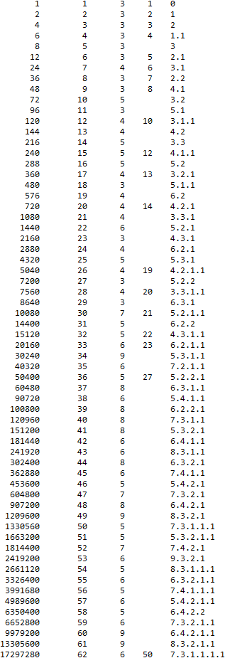
Table 5: A301414: m/A002110(A108602(m)) for m in A002182.
Smallest 60 terms k of A301414. (There are 2500 confirmed terms.)
(1) A301414(k) = m/A002110(A108602(m)) for m in A002182.
(2) k = index.
(3) A301415(k) = “Breadth” or 1 + nmax − nmin such that A002110(n) × A301414(k) is in A002182.
(4) If A301414(k) is in A002182 itself, its position in A002182 appears in this column.
(5) MN(A301414(k))..
Full dataset for A301414 and A301415 in OEIS b-file form.
Observations.
- Only 19 terms in the smallest 2500 are in A002182: {1, 2, 3, 4, 5, 6, 7, 8, 10, 12, 13, 14, 19, 20, 21, 22, 23, 27, 50}. Are there any more?
Table 6: Record setters in A301415.
(1) 1 + nmax − nmin.
(2) k (i.e., the horizontal location of the vertical length of non-white pixels that set records in Graph 4).
(3) nmin = least n such that A002210(n) × A301414(k) is in A002182.
(4)
nmax = greatest n such that A002210(n) × A301414(k) is in A002182.
(5) A301414(k).
(6) MN(A301414(k)).
Data file available. Text format, entries in columns (1) through (4) inclusive, delimited by spaces, each row by newline, 48 rows pertaining to the 8000 confirmed terms in A301415.
| i | (1) | (2) | (3) | (4) | (5) | (6) |
| --- | --- | ----- | ------------- | ---------------------------------- | ||
| 1 | 3 | 1 | 1 | 3 | 1 | 0 |
| 2 | 4 | 7 | 4 | 7 | 24 | 3.1 |
| 3 | 5 | 10 | 5 | 9 | 72 | 3.2 |
| 4 | 6 | 22 | 7 | 12 | 1440 | 5.2.1 |
| 5 | 7 | 30 | 9 | 15 | 10080 | 5.2.1.1 |
| 6 | 9 | 34 | 9 | 17 | 30240 | 5.3.1.1 |
| 7 | 10 | 74 | 21 | 30 | 129729600 | 6.4.2.1.1.1 |
| 8 | 13 | 77 | 19 | 31 | 259459200 | 7.4.2.1.1.1 |
| 9 | 14 | 98 | 25 | 38 | 10897286400 | 8.5.2.2.1.1 |
| 10 | 16 | 130 | 32 | 47 | 926269344000 | 8.5.3.2.1.1.1 |
| 11 | 17 | 136 | 31 | 47 | 1852538688000 | 9.5.3.2.1.1.1 |
| 12 | 19 | 145 | 33 | 51 | 7039647014400 | 9.5.2.2.1.1.1.1 |
| 13 | 21 | 150 | 35 | 55 | 17599117536000 | 8.5.3.2.1.1.1.1 |
| 14 | 23 | 154 | 33 | 55 | 35198235072000 | 9.5.3.2.1.1.1.1 |
| 15 | 25 | 170 | 40 | 64 | 404779703328000 | 8.5.3.2.1.1.1.1.1 |
| 16 | 30 | 176 | 38 | 67 | 809559406656000 | 9.5.3.2.1.1.1.1.1 |
Table 7: Tiers A002110(n) that set records for number of values A301414(k) such that A002110(n) × A301414(k) is in A002182.
(1) Record-setting number of families in A301414 that produce m in A002182.
(2) j = Tier n where (1) first occurs (i.e., the vertical location of the horizontal length of non-white pixels that set records in Graph 4).
(3) Least family (index in A301414) in record-setting range.
(4)
Greatest family (index in A301414) in record-setting range.
Data file available. Text format, entries in columns (1) through (4) inclusive, delimited by spaces, each row by newline, 48 rows pertaining to the 8000 confirmed terms in A301414.
| n | (1) | (2) | (3) | (4) |
| ---- | ----- | ----- | ----- | ----- |
| 1 | 1 | 1 | 1 | 1 |
| 2 | 2 | 2 | 1 | 2 |
| 3 | 5 | 3 | 1 | 5 |
| 4 | 6 | 4 | 2 | 7 |
| 5 | 12 | 5 | 3 | 15 |
| 6 | 16 | 7 | 7 | 22 |
| 7 | 19 | 9 | 10 | 34 |
| 8 | 21 | 10 | 16 | 40 |
| 9 | 23 | 12 | 22 | 45 |
| 10 | 30 | 17 | 34 | 68 |
| 11 | 31 | 19 | 39 | 77 |
| 12 | 33 | 22 | 48 | 91 |
| 13 | 36 | 25 | 60 | 104 |
| 14 | 46 | 31 | 77 | 136 |
| 15 | 47 | 33 | 88 | 154 |
| 16 | 48 | 37 | 92 | 161 |
| 17 | 58 | 55 | 150 | 222 |
| 18 | 66 | 63 | 170 | 272 |
| 19 | 67 | 64 | 170 | 272 |
| 20 | 94 | 67 | 176 | 290 |
| 21 | 98 | 69 | 192 | 320 |
| 22 | 99 | 93 | 297 | 419 |
| 23 | 102 | 188 | 561 | 713 |
| 24 | 104 | 190 | 583 | 738 |
| 25 | 108 | 192 | 596 | 738 |
| 26 | 124 | 206 | 638 | 805 |
| 27 | 130 | 218 | 656 | 861 |
| 28 | 133 | 271 | 864 | 1054 |
| 29 | 142 | 281 | 894 | 1095 |
| 30 | 150 | 463 | 1367 | 1609 |
| 31 | 164 | 547 | 1527 | 1757 |
| 32 | 168 | 726 | 1895 | 2210 |
| 33 | 173 | 738 | 1942 | 2273 |
| 34 | 188 | 763 | 2012 | 2285 |
| 35 | 194 | 787 | 2080 | 2369 |
| 36 | 208 | 835 | 2098 | 2531 |
| 37 | 213 | 910 | 2319 | 2783 |
| 38 | 223 | 942 | 2422 | 2908 |
| 39 | 235 | 991 | 2609 | 2958 |
Graph 8: Plot SHCNs at (A002110(n), A301416(k)) where index n pertains to A002110 and index k pertains to A301416.
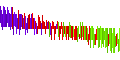
Let’s just focus on superior highly composite numbers, plotting them on a chart with the axis n = number of distinct prime divisors, and k the index of the primitive values of d with respect only to SHCNs. What we expect is a “single strand” sort of graph instead of a “river” of pixels.
This graph situates n on the horizontal axis and the multiplicity notation of familes k that produce m in A002201 on the vertical axis. We can reconstruct m = A002110(n) × k, with k decoded.
The graph below shows only SHCNs, eliminating the families k that do not produce SHCNs. The axes are flipped from Graph 4 such that the tiers n run horizontally, while the families k run vertically. The smallest 1024 SHCNs appear here. A larger map of the smallest 4096 SHCNs runs 3959 × 158 pixels.

The observations we would make regarding Graph 8 and its extension were laid out in Observation 4.4.
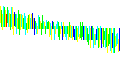
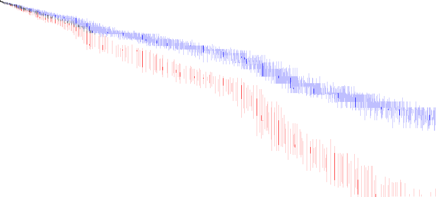
Graph 9: Plot HCNs and Superabundant Numbers.
The highly composite numbers and the colossally abundant numbers share many small values. Since the colossally abundant numbers are also products of primorials, we can also plot them on a similar graph. This time we use k as the index of the union of the set of primitive d pertaining to HCNs, and d pertaining to colossally abundant numbers.
The graph below shows the HCNs shown in Graph 4 in blue, and the superabundant numbers (i.e., numbers in A004394 that are also in A166735) in red. Numbers that are in both sequences (i.e., in A166981) are plotted black. The smallest 8436 superabundant numbers are shown, along with HCNs that are products of some primorial and MN(d) = "15.9.6.4.3.2.2.2.2.1.1.1.1.1.1.1.1.1.1.1.1.1.1.1.1.1.1.1", which would rank larger than A301414(1398).
Observations.
- The intersection of A002182 and A004394 is finite, with 449 terms. These appear at A166981. Thus the set of black pixels corresponds to the entire A166981 dataset.
- The largest term in A166981 is A002110(69) × A301414(192), but the term with the largest k is A002110(68) × A301414(202). These correspond to 69: 9.5.3.2.2.1.1.1.1 and 68: 9.5.3.2.1.1.1.1.1.1, respectively.
- The superabundant numbers generally tend to be products of larger primorials in select families d = A301414(k). None of the superabundant numbers have n lower than that which produce HCNs.
- A301414 is not sufficient to graph both A002182 and A004394. The first missing d = 592424239959167616000 → “10.5.3.2.2.1.1.1.1.1.1.1)” with regard to A301414 ranks between A301414(314) → “10.5.4.3.2.1.1.1.1.1.1” and A301414(315) → “10.6.3.2.2.2.1.1.1.1.1”. Consequently, the blue pixels to the right of the rightmost red line in the graph may not be plotted in the correct place; there most likely are additional vacant gaps in the blue stream of pixels that correspond to additional missing values of d in A301414.
- There is a marked "divergence" of A004394 in red from the direction of A002182 in blue around d = .
- Since we have not reached the full breadth of the red lines (i.e., vertical height, continuous range of primorials) that pertain to a given divisor d for the rightmost pixels, only the left 708 pixels of this data are validated. We could see additional red lines that are not accounted for, because the divisors d that produce them with larger primorials A002110(n) have not yet been encountered due to their magnitude.
- See this text table for the smallest 880 terms d of a sequence c(k) akin to A301414 that produces a HCN or superabundant number when multiplied with some primorial. In the table, we show the index of d in A301414 and a similar sequence b(k) such that d produces a number in A004394. This sequence c(k) is the union of A301414(k) (pertaining to blue data) and b(k) (pertaining to red data), and is the horizontal register of Graph 9.
The graph of m in A004394 as A002110(ω(m)) × d where d = m/A002110(ω(m)) will be the subject of a new data brief.
Graph 10: Superior highly composite and colossally abundant numbers.
Let’s relax the HCNs and the superabundant numbers and accentuate the superior highly composite numbers (A002201) and the colossally abundant numbers (A004490) in the above graph:
The graph below (10.1) is an enlargement of the above graph.
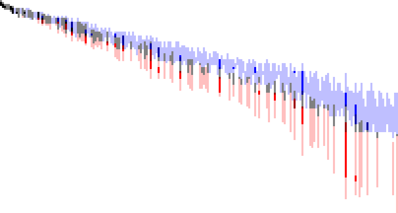
We note several kinds of numbers on this graph.
- Highly composite numbers that are not also superabundant appear in light blue.
- Superabundant numbers that are not highly composite are shown in pink.
- Superior highly composite numbers that are not superabundant appear in blue.
- Superior highly composite numbers that are also abundant but not colossally so (let’s call then SHCN-abundant) are in a darker tone of blue and are listed as part of A166981.
- Colossally abundant numbers not also highly composite are shown in red.
- Colossally abundant numbers that are also highly composite (let’s call them HCCA or highly composite-colossally abundant) appear in dark red and are also listed as part of A166981.
- There are 20 black pixels, numbers that are both SHCN and colossally abundant. These appear in black and are in A224078. The largest number plotted in black is 581442729886633902054768000 → 14: 10.5.4.2.1.1.
- Numbers that are both highly composite and abundant but neither highly composite and colossally abundant (i.e., the remaining terms of finite A166981) appear in gray. Together the 449 numbers in items 4 and 6, and this item comprise A166981.
Click here for an enlarged chart of Graph 10.1.
Observations.
Recall that U = A301414 = numbers d such that (d × p#) for some p# is in A002182. Let V = numbers d such that (d × p#) for some p# is in A004394 and let W = union(U, V). Since we are considering both numbers in A002182 and in A004394, we cannot rely solely on U or V to locate numbers in both sequences and their relatives A002201 and A004490, respectively, on a graph. Therefore, the d at k coordinate in the ordered pair pertains to W.
- Smallest number in A224078 = 2 → 1: 1.
- Largest number in A224078 = 581442729886633902054768000 → 17: 6.3.2.1 = 302400 p17#.
- k = 44 (d = 302400) has every flavor of number in the chart except SHCNs that are not superabundant.
- k = 176 (d = 809559406656000 → 9.5.3.2.1.1.1.1.1) is the largest k that has every flavor of number in the chart except numbers that are in A224078, i.e., numbers that are both SHCN and colossally abundant.
- Largest “gray” number (i.e., HCN that is abundant and in A166981) is A002110(68) × W(202).
- The number of “dark red” pixels is finite: there are 32 terms between (9, 20) and (66, 176). The smallest is A002110(9) × W(20) = 160626866400 → 9: 4.2.1. The largest “dark red” number (i.e., colossally abundant number that is also highly composite) is A002110(66) × W(176) → 66: 9.5.3.2.1.1.1.1.1, a 146 decimal digit number. This file lists the 32 “dark red” numbers in OEIS b-file format, while this file analyses the numbers in terms of prime divisors.
- The number of “dark blue” pixels is finite: there are 39 terms, between (8, 22) and (65, 187). The smallest is A002110(8) × W(22) = 13967553600 → 8: 5.2.1. The largest “dark blue” number (i.e., SHCN that is also superabundant) is A002110(65) × W(187) → 65: 10.6.3.2.1.1.1.1.1, a 144 decimal digit number. This file lists the 39 “dark blue” numbers in OEIS b-file format, while this file analyses the numbers in terms of prime divisors.
- There appears to be much agreement between the SHCNs and the colossally abundant numbers as to which k produce them. This seems to be increasingly falling out of register as we move down and right on the chart.
This graph (10.2) shows the superior highly composite numbers in blue, and the smallest 150 colossally abundant in blue, eliminating HCNs and abundant numbers that are neither superior highly composite nor colossally abundant. Here we flip the axes such that n increases horizontally rightward, and k increases vertically downward. Of course, regarding k, we are speaking of an index k of primitive values of divisors d = m/A002110(n) for m in A002201 or A004490, and not of A301414. The pixels in black show the 20 terms of A224078, numbers that are in both A002201 and A004490.
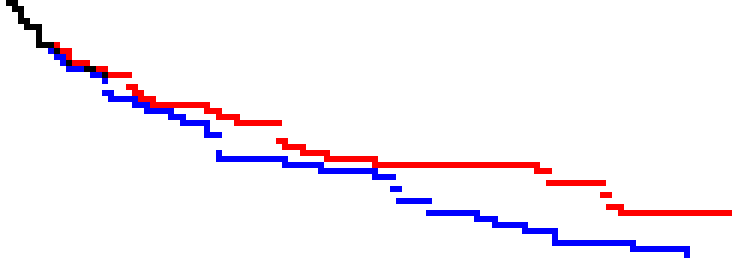
The graph (10.3) below extends this data to 1000 terms in A002201 (blue) and 1000 terms in A004490 (red). We use the 10,000 terms in A073751 to extend the 150 available terms of A004490:
Note the nearly parallel trajectories of the two sequences. This continues at least through the smallest 5000 terms each of A002201 and A004490. These graphs will be explored to a fuller extent in the future.
Code.
Mathematica code appears below if you would like to explore on your own.
A002182 Data: You must first download the b-file at A002182. Alternatively, use this Mathematica code to translate Achim Flammenkamp's data (renamed "HCN_124260.txt") to decimal:
Times @@ {Times @@ Prime@ Range@ ToExpression@ First@ #1, If[# == {}, 1, Times @@ MapIndexed[Prime[First@ #2]^#1 &, #]] &@
DeleteCases[-1 + Flatten@ Map[If[StringFreeQ[#, "^"], ToExpression@ #, ConstantArray[#1, #2] & @@ ToExpression@ StringSplit[#, "^"]] &, #2], 0]} & @@
TakeDrop[Drop[StringSplit@ #, 2], 1] & /@ Import["HCN_124260.txt", "Data"]
A002201 Data: The data furnished at A002201 only runs to 150 terms. If you want more, we can use the b-file at A000705 to get 10,000 terms:
a002201 = With[{s = Import["b000705.txt", "Data"][[All, -1]]}, FoldList[Times, s]]
A004394 Data: The data furnished in the b-file at A004394 includes 2000 terms decimally. We can convert the remaining, commented-out terms presented as products of primorials and factorials and get 8436 terms. First, make a b-file of the first 2000 terms, without the commented-out preamble. Then make a second b-file “b004394e.txt” only including the commented out terms 2001—8436. Then use the following function:
decode4394[w_] :=
Times @@ Flatten@ {Complement[#1, Union[#2, #3]],
Product[Prime@ i, {i, PrimePi@ #}] & /@ #2, Factorial /@ #3} & @@
ToExpression@ {StringSplit[w, _?(! DigitQ@ # &)],
StringCases[w, (x : DigitCharacter ..) ~~ "#" :> x],
StringCases[w, (x : DigitCharacter ..) ~~ "!" :> x]};
a004394 = Join[Import["b004394.txt", "Data"][[All, -1]], decode4394 /@ Import["b004394e.txt", "Data"][[All, -1]]];
There is a larger dataset produced by T. D. Noe with a million superabundant numbers. This dataset and A. Flammenkamp’s 779674-term HCN dataset will be employed in a future phase.
A054841 (MN): The multiplicity notation function:
A054841[n_] := If[n == 1, {0},
Function[f, ReplacePart[Table[0, {PrimePi[f[[-1, 1]] ]}], #] &@
Map[PrimePi@ First@ # -> Last@ # &, f]]@ FactorInteger@ n];
Graph 4: Produce a text-style graph (good for small samples of the entire dataset).
Block[{s = Import["b002182.txt", "Data"][[All, -1]], a, b, c, m, u},
s = Take[s, 1000];
a = Array[{#2, #1, StringTrim[StringReplace[ToString@ #, ", " -> "."], ("{" | "}") ...] &[#3 /. {} -> 0],
Times @@ MapIndexed[Prime[First@ #2]^#1 &, #3]} & @@
{#1, Boole[First@ #2 > 0] Length@ #2, DeleteCases[-1 + #2, 0] /. -1 -> 0} & @@
{s[[#]], A054841@ s[[#]]} &, Length@ s];
u = Function[{t, k}, Map[StringPadRight[#, k] &, t]] @@ {#, Max@ Map[StringLength, #]} &@
Map[StringTrim[StringReplace[ToString@ A054841@ #, ", " -> "."], ("{" | "}") ...] &, Union@ a[[All, -1]] ];
b = MapIndexed[{i_, j_, k_, #1} -> ToExpression@ StringJoin["{i,", ToString@ First@ #2, ",", " j, k}"] &,
Union@ a[[All, -1]]]; c = Map[# /. b &, a]; m = Max[c[[All, 2]] ];
c = Map[Sort@ # &, SplitBy[SortBy[c, First], First]];
MapIndexed[u[[First@ #2]]~StringJoin~StringJoin[#1] &,
Transpose@ Array[With[{t = ConstantArray[" ", m]},
ReplacePart[t, Map[#2 -> "x" & @@ # &, c[[#]] ]] ] &, Length@ c]] ] // TableForm
Graph 4: Produce an image of Graph 4:
Block[{s = Import["b002182.txt","Data"][[All,-1]], a002201 = Import["b002201.txt","Data"][[All,-1]], a, b, c, m, u},
a = Array[{#2, #1, StringTrim[StringReplace[ToString@ #, ", " -> "."], ("{" | "}") ...] &[#3 /. {} -> 0],
Times @@ MapIndexed[Prime[First@ #2]^#1 &, #3]} & @@ {#1, Boole[First@ #2 > 0] Length@ #2,
DeleteCases[-1 + #2, 0] /. -1 -> 0} & @@ {s[[#]], A054841@ s[[#]]} &, Length@ s];
u = Function[{t, k}, Map[StringPadRight[#, k] &, t]] @@ {#, Max@ Map[StringLength, #]} &@
Map[StringTrim[StringReplace[ToString@ A054841@ #, ", " -> "."], ("{" | "}") ...] &, Union@ a[[All, -1]] ];
b = MapIndexed[{i_, j_, k_, #1} -> ToExpression@ StringJoin["{i,", ToString@ First@ #2, ", j, k}"] &, Union@ a[[All, -1]]];
c = Map[# /. b &, a];
m = Max[c[[All, 2]] ];
c = Map[Sort@ # &, SplitBy[SortBy[c, First], First]];
Image[Array[With[{t = ConstantArray[{1, 1, 1}, m]},
ReplacePart[t, Map[#2 -> If[FreeQ[a002201, #3], {0, 0, 0}, {1, 0, 0}] & @@ # &, c[[#]] ]] ] &, Length@ c], ColorSpace -> "RGB" ] ]
Graph 9: Produce an image of Graph 9:
Block[{r, s = a004394, t, u, v, a, b},
t = TakeWhile[a002182, # <= Max@ s &]; u = Union[s, t];
a = Array[{#1, #2, #1/Product[Prime@ i, {i, #2}]} & @@ {u[[#]],
PrimeNu[u[[#]] ]} &, Length@ u]; v = Union[a[[All, -1]] ];
b = Array[{#2, #3,
FromDigits[{1 - Boole@ FreeQ[s, #1], 1 - Boole@ FreeQ[t, #1]},
2]} & @@ {#1, #2, FirstPosition[v, #3][[1]]} & @@ a[[#]] &,
Length@ a];
r = ConstantArray[{1, 1, 1}, Max[b[[All, 2]] ] ];
Image[#, ColorSpace -> "RGB"] &@
Array[ReplacePart[r,
Map[#1 -> Which[#2 == 1, {0, 0, 1}, #2 == 2, {1, 0, 0}, True, {0, 0, 0}] & @@ # &,
With[{k = #}, Select[b, First@ # == k &]][[All, {2, 3}]] ] ] &, 1 + Max[b[[All, 1]] ], 0] ]
Terms stored in the graphs: Produce an image of Graph 4 from the .png! (use the filename of the image; this filename pertains to a small image; note that graphs supported by this code are only those that show HCNs and SHCNs):
With[{i =
ImageData[
Import["HCN1.png", "PNG"]] /. {{0., 0., 0.} -> 1, {1., 1., 1.} -> 0, {1., 0., 0.} -> 1}},
Sort@ Map[Product[Prime@ k, {k, #1 - 1}] a301414[[#2]] & @@ # &, Position[i, 1]]]
A301413: A002182(n) / A002110(A108602(n)).
With[{s = Import["b002182.txt", "Data"][[All, -1]]},
Array[#/Product[Prime@ i, {i, PrimeNu[#]}] &@ s[[#]] &, 62]]
A301414: Values k in A301413 such that k × A002110(m) is in A002182. (proposal pending)
With[{s = Import["b002182.txt","Data"][[All,-1]] *)},
Union@ Array[#1/Product[Prime@ i, {i, #2}] & @@ {#, PrimeNu@ #} &@ s[[#]] &, Length@ s] ]
A301415: Number of terms m in A002110 such that A301413(k) × A002110(m) is in A002182. (to be proposed if A301414 is accepted)
Block[{s = a002182, a, b, c, m, u},
a = Array[{#2, #1, StringTrim[StringReplace[ToString@ #, ", " -> "."], ("{" | "}") ...] &[#3 /. {} -> 0], Times @@ MapIndexed[Prime[First@ #2]^#1 &, #3]} & @@ {#1, Boole[First@ #2 > 0] Length@ #2,
DeleteCases[-1 + #2, 0] /. -1 -> 0} & @@ {s[[#]], A054841@ s[[#]]} &, Length@ s];
u = Union@ a[[All, -1]] (* A301414 *);
b = MapIndexed[{i_, j_, k_, #1} -> ToExpression@ StringJoin["{i,", ToString@ First@ #2, ",", " j, k}"] &, Union@ a[[All, -1]]];
c = Map[# /. b &, a];
m = Max[c[[All, 2]] ];
c = Map[Sort@ # &, SplitBy[SortBy[c, First], First]];
Total /@ Transpose@ Array[With[{t = ConstantArray[0, m]}, ReplacePart[t, Map[#2 -> 1 & @@ # &, c[[#]] ]] ] &, Length@ c] ]
A301416: Numbers m such that m × A002110(k) is in A002201 for some k. (to be proposed if A301414 is accepted)
Block[{s = a002201(*Import["b002201.txt","Data"][[All,-1]]*)}, s = Take[s, 250];
Union@ Array[Times @@ MapIndexed[Prime[First@ #2]^#1 &, #3] & @@ {#1, Boole[First@ #2 > 0] Length@ #2, DeleteCases[-1 + #2, 0] /. -1 -> 0} & @@ {s[[#]], A054841@ s[[#]]} &, Length@ s]]
Contact me on LinkedIn if you desire other programs I’ve used to generate this file for your own research.
Thus concludes our excursion regarding Ramanujan’s highly composite numbers.
Dedication.
This work is dedicated to my father, Thomas De Vlieger, who had supported my computer science interests first with that 64k RAM Apple II+ in December 1980. It is by having this machine that I learned Applesoft BASIC on my own at ages 10-12 and taught myself how to program. It would not have happened were it not for his foresight, as I wanted to be an astronomer, and ended up majoring in architecture. Obviously his intuition demonstrated a level of knowledge of my true interests that proved even more honest and true than my own. Thank you Dad, and I love you.
Acknowledgements.
Many thanks are owed to Achim Flammenkamp for my long-standing interest in the data he’d generated regarding the highly composite numbers, especially my use of OEIS A054841 to abbreviate highly composite and highly regular numbers.
Thanks are also in order for Dr. Neil Sloane and the OEIS for its ready availability of the mindshare of mathematical knowledge made available freely to the world. I had been interested in sequences since age 17 via references in the CRC Standard Math Tables, 28th Edition. It is through the OEIS that I attained fluency in Mathematica, and none of this work would thus be possible.
Concerns sequences:
A000005: Divisor counting function τ(n).
A000705: A002201(n) is product of first n terms of this sequence.
A001221: ω(n) = Number of distinct prime divisors of n.
A002110: The primorials.
A002201: Superior highly composite numbers (SHCNs).
A002182: Highly composite numbers (HCNs), i.e., where records are set in A000005.
A002183: Records in A000005 = A000005(A002182(n)).
A004394:
Superabundant numbers: n such that σ(n)/n > σ(m)/m for all m < n.
A004490: Colossally abundant numbers.
A025487: List giving least integer of each prime signature; also products of primorial numbers.
A051903: Maximal exponent in prime factorization of n; greatest term in MN(n).
A054841: For n = Product_pe, write ek in the k-th place, or write 0 if pk does not divide n.
A055932: Numbers where all prime divisors are consecutive primes starting at 2.
A060735: Irregular triangle read by rows: T(n, k) = k × A002110(n) for 1 ≤ k < prime(n + 1).
A073751: Prime numbers that when multiplied in order yield the sequence of colossally abundant numbers.
A108602: A001221(A002182(n)).
A112779: Largest exponent in the prime factorization of highly composite numbers.
A166735:
Superabundant numbers (A004394) that are not highly composite (A002182).
A166981:
Superabundant numbers (A004394) that are highly composite (A002182).
A224078: Numbers that are superior highly composite and colossally abundant.
A244052: Highly regular numbers, i.e., where records are set in A010846.
See [3] for these and other A-number sequences in this work.
References.
[1]: Achim Flammenkamp, “Highly Composite Numbers”, retrieved 2018 0329 2330 GMT. Downloads appear at the bottom of page and require “gunzip” application.
[2]: D. B. Siano, J. D. Siano, “An Algorithm for Generating Highly Composite Numbers.”, 1994.
[3]: Neil Sloane, The Online Encyclopedia of Integer Sequences, retrieved 2018 0329 2330 GMT. See “Concerns Sequences” for individual links.
[4]: Eric Weisstein’s World of Mathematics, “Highly Composite Number”, retrieved 2018 0403 1715 GMT.
General references:
L. Alaoglu, P. Erdös, On highly composite and similar numbers, Transactions of the American Mathematical Society 56 (1944), pp. 448-469. (Theorem 3 largest prime factor, 4 page 456 two with i = 2 for pi, product of primorials.)
Srinivasa Ramanujan, Highly composite numbers, Ramanujan Journal 1 (1997), p. 119-153.
Original text-format data brief can be seen here.
Document Revision Record.
2018 0328 1015 Created.
2018 0328 2030 Table 3 added.
2018 0331 0845 Data brief converted to HTML; portion ascribed to A301413 partitioned.
2018 0331 1415 Improved tables and charts.
2018 0331 2230 Added several tables, abstract, and other material.
2018 0401 0815 Extended Table 6.
2018 0401 1130 Added Table 7.
2018 0401 1200 Added Code.
2018 0401 1615 Added Graph 8 and code for new A-numbers.
2018 0401 2030 Added proposed sequences, data, and code pertaining to such.
2018 0403 1745 Added references [2] and [4], and sequence A112779.
2018 0405 1715 General edit, detailed analysis of Graph 4.
2018 0409 1800 Proposal of A301414-A301416, Graph 9.
2018 0411 1130 General edit.
2018 0413 1630 Added Graphs 10, 10.1, 10.2.
2018 0414 0815 Corrected Graph 10, added 10.1, renumbered 10.1 and 10.2.
2018 0417 1730 Added observations to Graph 10.1.
2018 0424 2100 Processing of 779674 HCNs and extension of Graph 4.
2018 0425 1045 Table 6 and 7 datasets.
2018 0428 1700 Final edit.
(Updated 28 April 2018)