OEIS A008336
A sequence by Bernardo Recamán Santos, this page written by Michael Thomas De Vlieger, St. Louis, Missouri, 2020 0912.
Abstract.
An examination of the Recamán sequence OEIS A008336, inspired by Scott R. Shannon’s A337486. We also compare A008336 to Paul Tek’s A260850 and Labos Elemer’s A055204. We recognize that a(n) = A008336, u(n) = A260850, and s(n) = A055204(n), generally considered f(n), are self-referential sequences conditioned on x | f(n − 1), if true f(n) = f(n − 1)/x, else f(n) = f(n − 1) × x. Let n = p1e1 × p2e2 × … × pkek, the standard form prime decomposition of n. The sequence a(n) is based on the condition n | a(n − 1), while u(n) is based upon u(n − 1) | pkek for all prime power divisors pkek | n, and s(n) upon s(n − 1) | p for all prime divisors p | n with multiplicity. We see u(n) as a version of a(n) that allows each prime power divisor to interact with the previous term independently. We show that s(n) is an atomized version of a(n) and u(n) that allows us to dispense with conditions and instead, for s(n − 1) → s(n) have each multiplicity ek(n) = ek(n − 1) + (ek mod 2) mod 2 for all pk | n with multiplicity. We plot the sequences and examine the multiplicities in their prime power decompositions using A067255.
Introduction.
This work examines the prime decomposition of a(n) in “multiplicity notation,” M(n) = A067255(n), and the numbers that induce a decrease in a(n), i.e., those places where a(n) exceeds a(n + 1), i.e., where a(n + 1) = a(n)/n. The indices of the decreases in a(n) are in b(k) = A337486(n), a sequence by Scott R. Shannon.
Let a(n) = A008336(n + 1) be the sequence starting from a(1) = 1 defined as follows:
if n | a(n − 1),
then a(n) = a(n − 1)/n,
else a(n) = a(n − 1) × n.
The sequence a(n) for our purposes begins: (See Code 1.1 and Code 1.2)
{1, 2, 6, 24, 120, 20, 140, 1120, 10080, 1008, 11088, 924, 12012, 858, 12870, 205920, 3500640, 194480, 3695120, 184756, 3879876, 176358, 4056234, 97349616, 2433740400, 93605400, 2527345800, 90262350, ...}
(We offset from the OEIS index here so as to juxtapose the condition n with the resultant operation a(n), merely as a convenience; we do not mean to argue alteration of the OEIS offset, which was put into effect for good reason there.)
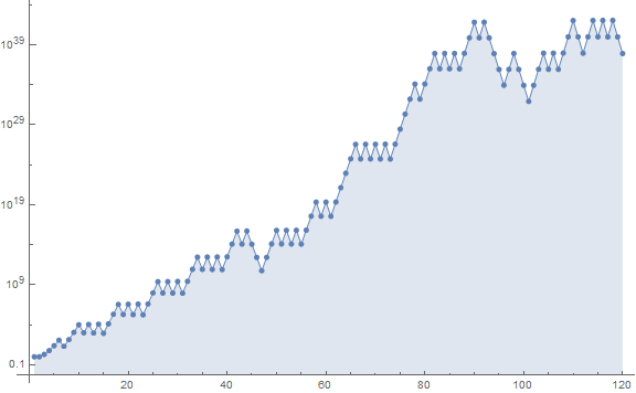
Figure 1.1 plots a(n) for 1 ≤ n ≤ 120 scaling y = log(a(n)):
(compare to Figures 4.4 and 5.1.)
We see that the advances and retreats appear to land near the same points in the plot, but this is an illusion; they land close to the same numbers. Example: the first dithering begins at n = 17:
n a(n)
------------
17 3500640
18 194480
19 3695120
20 184756
21 3879876
22 176358
23 4056234
The increasing highs and decreasing lows seem to reflect similar behavior of Recamán’s more famous sequence A005132, however not as frequently repeated as in A005132.
Figure 1.2 is a log plot of a(n) for 1 ≤ n ≤ 1000:
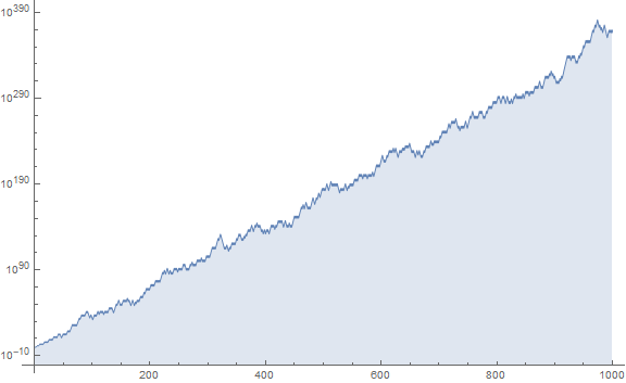
The graph shows the advances and retreats in aggregate, that there are sometimes sustained runs of falls and rises.
Figure 1.3 below shows the records in red, the local minima in black, decreasing points in green, and the rest of the points in blue:
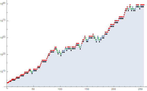
The sequence b(k) contains all n | a(n − 1), a condition that triggers division and necessarily reduces a(n) toward a local minimum in isolation, but when in runs, e.g., for 92 ≤ n ≤ 96, we see a downward trend and only n = 95 is a local minimum. The numbers in b(k) are plotted in both green and black in Figure 1.3.
The sequence b(k) begins: (See Code 1.3.)
{6, 10, 12, 14, 18, 20, 22, 26, 28, 30, 34, 36, 38, 42, 44, 45, 46, 50, 52, 54, 58, 60, 66, 68, 70, 72, 78, 82, 84, 86, 90, 92, 93, 94, 95, 98, 99, 100, 104, 106, 110, 111, 114, 116, 118, 119, 122, 124, 126, 130, ...}
Many of these but not all are local minima; those terms that are local minima appear in bold above. Figure 1.3 shows the downard moves in green; when they reach a local minimum, the figure plots it in black.
We find runs of n that divide a(n). For example, 44 | a(43) = 5207644935207000, 45 | a(44) = 118355566709250, and 46 | a(45) = 2630123704650, triggering three successive decreases in a(n). Table 1.1 below shows the terms k1…k2 of b(k) with 1 ≤ k ≤ 4740516 that have run length ℓ such that k1 is the least k that starts a such a run of length ℓ:
Table 1.1.
ℓ run of consecutive terms in b(k)
--------------------------------------------------------
2 110, 111
3 44, 45, 46
4 92, 93, 94, 95
5 986, 987, 988, 989, 990
6 1025, 1026, 1027, 1028, 1029, 1030
7 322, 323, 324, 325, 326, 327, 328
8 18024, ..., 18031
9 8198, ..., 8206
10 21505, ..., 21514
11 192067, ..., 192077
12 992195, ..., 992206
13 1873412, ..., 1873424
14 4995146, ..., 4995159
...
Records Transform of a(n).
A similar analysis of upward moves and records in a(n) might be pursued. Apart from the records transform, we will focus instead on downward moves in a(n) which are linked with the occasion where n | a(n − 1) and are thereby interesting.
The records r(k) set by a(n) as n increases begins with the following (shown in Figure 1.3 by red points):
1, 2, 6, 24, 120, 140, 1120, 10080, 11088, 12012, 12870, 205920, 3500640, 3695120, 3879876, 4056234, 97349616, 2433740400, 2527345800, 2617608150, 2704861755, 86555576160, 2856334013280, 2940343837200, 3022020054900, ...
The sequence s(k) contains indices of records r(k) in a(n), again, differing from the index of A008336 in OEIS, in that they are 1 less than that of A008336:
1, 2, 3, 4, 5, 7, 8, 9, 11, 13, 15, 16, 17, 19, 21, 23, 24, 25, 27, 29, 31, 32, 33, 35, 37, 39, 40, 41, 43, 49, 51, 53, 55, 56, 57, 59, 61, 62, 63, 64, 65, 67, 69, 71, 73, 74, 75, 76, 77, 79, 80, 81, 83, 85, 87, 88, ...
The indices written this way versus that of the OEIS convey multipliers such that a(n) sets a record.
Multiplicity Notation.
This work aims to analyze the prime decomposition of a(n) when we have the condition n | a(n − 1). Of course, standard form prime decomposition may be used. For example regarding n = 84, his is the familar 84 = 2² × 3 × 7. Because of the magnitude of the numbers we wish to examine and the quantity of data we shall consider, we adopt an abbreviated form of this notation.
Let M(n) = A067255(n) be the exponents e of the prime power divisors pe | n written in position π(p) little-endian fashion beginning with the least p, including primes q that do not divide n that interpose between the least prime factor p = lpf(n) and the greatest prime factor p = gpf(n). Unfilled positions π(q) for q > gpf(n) are presumed to be 0 as opposed to null. Example, for n = 84 = 2² × 3 × 7, we write 2.1.0.1, here delimiting the multiplicities by dots. We render the empty product n = 1 as M(1) = 0.
For n < 210 = 1024, we may simply concatenate this expression to be “2101” for concision (in the fashion of A054841(n) in reverse), or we may replace the medial zero with a dot to as to read these zeros as “21.1”. This latter concatenation approach becomes ambiguous for multiplicities that exceed 9, therefore herein we use it for sake of explanation, but in code we allow exponents to be expressed distinctly and not in a concatenated way.
The Multiplicity Register of a(n).
Let’s look at the first few terms of a(n) and M(a(n)), for concision, using the concatenation form of the latter, with asterisks marking the condition n | a(n − 1). The last column is M(n), with a dash in front signifying that the multiplicities are subtracted from their corresponding positions in M(a(n)): (See the appendix for an extended table of multiplicities. See Code 2.1.)
Table 2.1
n a(n) M(a(n)) M(n)
----------------------------
1 1 0 0
2 2 1 1
3 6 11 .1
4 24 31 2
5 120 311 ..1
6* 20 2.1 - 11
7 140 2.11 ...1
8 1120 5.11 3
9 10080 5211 .2
10* 1008 42.1 - 1.1
11 11088 42.11 ....1
12* 924 21.11 - 21
13 12012 21.111 .....1
14* 858 11..11 - 1..1
...
a(n) Seen as a Constructor of n in b(k).
We note application of index n in this way (as opposed to the OEIS index at A008336) allows us to examine the multiplicities of the prime factors of n and a(n) as a fit between M(a(n)) and M(n).
In this way we may assemble sequence b(n) by storing all n | a(n) that trigger the a(n)/n condition.
Examples:
Given a(n) = 1,
We see n = 2 does not divide a(n − 1) = 1, thus a(2) = 1 × 2 = 2.
We see n = 3 does not divide a(n − 1) = 2, thus a(3) = 2 × 3 = 6.
The number n = 4 does not divide a(n − 1) = 6, thus a(4) = 6 × 4 = 24.
Prime n = 5 does not divide a(n − 1) = 24, thus a(5) = 24 × 5 = 120.
Composite n = 6 | a(n − 1) = 120, thus a(5) = 120/6 = 20, etc.
It is clear that for n = p prime, a(p) = a(p− 1) × p, since hitherto, the factor p has not yet produced a term in a(n). Therefore, all the terms of a(n) are composite.
We might also look at a(n) instead as a register where Ri stores the multiplicities of prime pi, with a(n) being the product of all the pi^Ri. Thus, we revisit the examples to look at a(n) as a register:
Given a(n) = 1, the empty product, all the Ri are set to 0,
For n = 2, we need one 2, but R1 = 0, thus we set R1 = 1.
For n = 3, we need one 3, but R2 = 0, thus we set R2 = 1; now the register reads “1,1”, since R1 = R2 = 1.
For n = 4 = 2 × 2, we need two 2s but only have 1 in R1, so we dump both into R1. Now the register reads “3,1”.
Prime n = 5 requires one 5, but R3 = 0, thus we set R3 = 0. Now the register reads “3,1,1”.
For n = 6, we need one 2 and one 3 and have both of these in the register! So we write 6 as the first term of b(k), and withdraw the primes from the register by decrementing R1 and R2. This depletes the 3s! Now the register reads “2,0,1”.
From what has happened to the 3s in the register in the example above, we know the next time we need any 3s, we’ll come up short, and whatever primes that divide that number, with multiplicity, will enter the register. In this case, it is 9 that will pass into the register. We also know that since 7 is prime, it will also enter the register, as will the three 2s that produce 8, since we only have 2. For n = 9, the register should read “5,2,1,1”. This is sufficient for n = 10 to enter b(k), leaving the register to read “4,2,0,1”, depleting the 5s, meaning that 15 will not be found in b(k), etc.
The Behavior of the Register.
Since we may credit multiplicity but also withdraw, the register Ri pertaining to any given prime pi may be totally depleted, and the depletions will be episodic. If Ri is in a state of depletion when n is a perfect prime power pie, we recharge Ri = e. Indeed the occasion of a perfect prime power pie constitutes either a large withdrawal or a large deposite in the register Ri.
Since we often have a composite number n that is not a perfect prime power, the depletion of Ri affects the behavior of the registers of other primes, and thereby the passage of n into b(k).
We have seen that n = 6 depleted the 3s so as to prevent 9 to enter b(k), and the depletion of 5s by n = 10 spelling doom for n = 15 in b(k). For n = 30, we see the depletion of 2s, setting the stage for a windfall of 2s delivered by n = 32:
Table 3.1
n register
----------------
29 152...1111
30 * .41...1111
31 .41...11111
32 541...11111
We also note the run of depleted registers R for 4 ≤ i ≤ 6.
Credits, Withdrawals, Runs, and Bridges.
We have seen that n = pi initializes the register Ri = 1. This has two consequences.
Firstly, p | a(p), and prevprime(n) | a(n) for composite n, where prevprime(n) is the largest prime less than n. Indeed, p is the greatest prime factor of a(n) in both cases. Therefore, gpf(a(n)) = prime(π(n)) for n > 1.
Secondly, we see structure in the plot of the register or the multiplicities of primes in a(n). Generally, we deplete Ri for n = 2p if and only if R1 is not also depleted. If there are no 2s to build 2pi, instead of depleting Ri, it increments to 2. This first occurs for i = 11, since at n = 60, we have depleted the 2s:
Table 3.2
n register
----------------
n V
60 * ...31.11..1111111
61 ...31.11..11111111
62 1..31.11..21111111
63 12.41.11..21111111
64 72.41.11..21111111
65 72141111..21111111
... |
90 * 42332.121122..1111111111
91 423421121122..1111111111
92 * 22342112.122..1111111111
93 * 21342112.112..1111111111
94 * 11342112.112...111111111
95 * 11242111.112...111111111
Here, indicated by “V”, we see the bridging of R11 (pertaining to prime 31) from n = 62 (where R1 was depleted) to n = 93 = 3 × 31.
When 2p is successful in entering b(k), the depletion of Ri follows that of registers of immediately-smaller primes so as to produce a run of depleted registers that would generally be recharged at n = 3p. The runs of depleted registers feature temporary “bridges” of doubly-strong registers that persist usually until the next block of 1s in the registers. Whether or not we have Ridepleted or Ri = 2, for n = 3pi sets Ri = 1. The interference of Ri by other primes becomes more complicated as the multiplier kpi increases.
We note that the register sometimes features a number of “leading zeros”, which, given the little-endian notation, indicates that we might find numbers in a(n) that have least prime factors other than 2. Indeed, the first odd term we see is a(30) = 87253605; this is the point where n = 30, via a(29)/30, depletes R1 in the register as seen in Table 3.1. We may also find numbers that are indivisible by primorial pj# = A002110( j). Table 3.3 lists j, followed by n and a(n) for n ≤ 66560:
Table 3.3:
j n a(n) M(a(n))
--------------------------------------------
1 2 2 1
2 30 87253605 .41...1111
3 55 6692604275665385 ..121.1..1111111
4 54 121683714103007 ...2..1..1111111
...
In contrast, we are able to find terms in b(k) that are indivisible by pj# across a wider range of j:
j p_j k b(k) M(b(k))
-------------------------------------------------
1 2 1 6 11
2 3 16 45 .21
3 5 35 95 ..1....1
4 7 46 119 ...1..1
5 11 272 649 ....1...........1
6 13 99 247 .....1.1
7 17 117 289 ......2
8 19 581 1349 .......1...........1
9 23 283 667 ........11
10 29 460 1073 .........1.1
11 31 572 1333 ..........1..1
12 37 589 1369 ...........2
13 41 727 1681 ............2
14 43 1113 2537 .............1..1
15 47 1470 3337 ..............1....1
16 53 1561 3551 ...............1..1
17 59 1912 4307 ................1...1
18 61 1636 3721 .................2
19 67 1993 4489 ..................2
20 71 2500 5609 ...................1.1
21 73 2574 5767 ....................11
22 79 3436 7663 .....................1..1
23 83 3089 6889 ......................2
24 89 3549 7921 .......................2
...
We observe these are squares or squarefree semiprimes (with exception of b(16) = 45). When p² is not in b(k), is it always so that we can find pq for some prime q? The occasion of a number n in b(k) precipitates from n | a(n − 1). For b(k) with 1 ≤ k ≤ 4740516, the largest least prime found is p(446) = 3137 | 9840769, the latter being the square of the former.
In aggregate this makes for an interesting plot.
The maximum multiplicity in the register has the following records set at the listed indices n; this data would help calibrate a heat map of multiplicities and so appears here. The maximum multiplicity indicated in column “Max*” is found in Rk, for example, for i = 10, a(705) has R3 = 13 therefore is divisible by the factor p313 = 513. This covers 1 ≤ n ≤ 216:
Table 3.4:
i n Max* k a(n)
-------------------------------------------------
1 2 1 1 2
2 4 3 1 24
3 8 5 1 1120
4 64 7 1 5522972043062121321953664
5 192 8 1 2611223349855351631199749777071371365036347123183195863161883821824
6 243 9 2 ...
7 309 10 2
8 315 11 2
9 504 12 2
10 705 13 3
11 720 14 3
12 725 16 3
13 750 17 3
14 755 18 3
15 800 19 3
16 2754 23 2
17 2757 24 2
18 2817 25 2
19 4032 26 2
20 4035 27 2
21 4041 28 2
22 14799 29 2
23 14805 30 2
24 14808 31 2
25 14811 32 2
26 14949 34 2
27 14952 35 2
28 14955 36 2
29 22473 37 2
30 22518 38 2
31 22521 39 2
32 22524 40 2
33 22527 42 2
34 43353 44 2
35 60201 45 2
...
Plot of the Register.
Figure 3.1 plots n on the x axis and the multiplicities in the registers on the y axis. The plot is color-coded to show the multiplicity 1 as beige, 2 as chartreuse, 3 a kelly green, 4 as cyan, etc. into blues, with 9 as red. The black bars indicate n in b(k). (View a large plot of 1 ≤ n ≤ 214 here.)

The plot shows an oscillation for R1 (pertaining to 2), the bottommost row of pixels, that breaks down into a more complex pattern as n increases. Similar oscillations seem to occur for fewer cycles at R2 and R3, but these receive interference from other registers. Of course, R11 is tweaked by the depletion of 2 for n = 62; this is the lower of the two chartreuse horizontal streaks furthest out above the action to the left.
Figure 3.2 zooms out to include 1 ≤ n ≤ 1024 (See Code3.1):

(compare to Figure 4.7 or Figure 5.3)
Figure 3.3 is a grayscale version of Figure 2:

Alternative to the graphic plot is a textual plot that is too large to include here, but can be seen in this text file, containing the multiplicities in the register for 1 ≤ n ≤ 1024.
Unraveling the Register Plot.
What happens if we “unfold” the plot so that the multiples kp are aligned? We know that for any register Rk that pertains to the k-th prime, the multiplicity changes only when we encounter n = kp. Therefore we may justify the “stripes” in the plot above and compare the behavior of a(n) for n = kp across all primes p. Indeed, without interference from any other prime, the multiplicities registered for p > 2 would oscillate between 1 and 0 as we increment k, until k = p, therafter we would have oscillation between 2 and 1. (See Code 4.1 and Code 4.2.)
Table 4.1:
k\p 2 3 5 7 11 13 17 19 23 29 31 37 41 43 47 53 59 61 67 71 73 79 83 89 97 01 03 07 09 13 27 31 37 39 49 51
---------------------------------------------------------------------------------------------------------------
1 1 1 1 1 1 1 1 1 1 1 1 1 1 1 1 1 1 1 1 1 1 1 1 1 1 1 1 1 1 1 1 1 1 1 1 1
2 3 . . . . . . . . . 2 2 . . . . . . . . . . . . . . . . 2 . . . . . . .
3 2 2 1 1 1 1 1 1 1 1 1 1 1 1 1 1 1 1 1 1 1 1 1 1 1 1 1 1 1 1 1 1 1 1 1 1
4 5 1 . . . . . 2 . . . . . . 2 . . . 2 . . 2 2 . . . . . . . . . . . . .
5 4 2 2 1 1 1 1 1 1 1 1 1 1 1 1 1 1 1 1 1 1 1 1 1 1 1 1 1 1 1 1 1 1 1 1 1
6 2 . 1 . . . 2 . 2 2 . . . . . . . . . . . . . . . . . . . . . . . . . .
7 1 1 2 2 1 1 1 1 1 3 1 1 1 1 1 1 1 1 1 1 1 1 1 1 1 1 1 1 1 1 1 1 1 1 1 1
8 5 2 3 3 2 . . 2 . 2 2 2 . . . . . . 2 2 2 . 2 . . 2 2 2 2 . . 2 . . 2 2
9 4 5 2 4 1 1 1 1 1 1 3 1 1 1 1 1 1 1 1 1 1 1 1 1 1 1 1 3 1 1 1 1 1 1 1 1
10 2 4 . 3 . . . . . . 2 . . . . . 2 . . . . . . 2 . . . 2 . . . . . . . .
11 1 5 1 4 2 1 1 1 1 1 3 1 1 1 1 1 1 1 1 1 1 1 1 1 1 1 1 1 1 1 1 1 1 1 1 1
12 4 3 . 3 1 . . 2 . 2 2 . . . . 2 . . . . . 2 . 2 . 2 . . 2 2 . . . . . .
13 3 4 1 4 2 2 1 1 1 1 3 1 1 1 1 1 1 1 1 1 1 1 1 1 1 1 1 1 3 1 1 1 1 1 1 1
14 1 3 . 2 1 3 . . . 2 2 . . . . . . . . . . . . 2 . . . . 4 . . . . . . 2
15 . 1 2 3 . 4 1 1 1 1 1 1 1 1 1 1 1 1 1 1 1 1 1 1 1 1 1 1 3 1 1 1 1 1 1 1
16 5 2 3 4 1 5 2 2 2 2 2 . . 2 2 2 2 . 2 2 . 2 . . 2 . 2 2 4 2 2 2 2 2 2 2
17 4 3 4 3 2 6 . 1 1 1 1 1 1 1 3 1 1 1 1 3 1 1 1 1 1 1 3 3 5 1 1 1 3 1 3 3
18 2 . 3 2 1 7 1 . . . . . . . 2 . . . . 2 . 2 . . . . 2 2 4 . . . 4 . 2 4
19 1 1 2 3 2 6 . 2 1 1 1 1 1 1 3 1 1 1 1 1 1 3 1 1 1 1 1 1 3 1 1 1 3 1 1 3
20 4 . . 4 3 5 1 3 2 . 2 . . . 4 . . . 2 2 . 4 . . . 2 . 2 2 2 . . 2 . . 4
21 3 2 1 2 2 4 . 2 1 1 1 1 1 1 3 1 1 1 1 1 1 3 1 1 1 1 1 1 3 3 1 1 1 1 1 3
22 1 1 . 1 . 3 1 1 . 2 . . . 2 2 . . . . . . 4 . . . . . 2 2 2 . 2 . . . 4
23 . 2 1 . 1 4 . 2 2 1 1 1 1 1 1 1 1 1 1 1 1 3 1 1 1 1 1 1 1 1 1 1 1 1 1 3
24 4 . 2 1 . 3 1 1 3 . 2 . 2 . . 2 . . . . 2 2 . . 2 . . . 2 2 2 . 2 . . 2
25 3 1 5 . 1 2 2 2 2 1 1 1 1 1 1 1 1 1 1 1 3 1 1 1 1 1 1 1 1 3 1 1 3 1 1 1
26 1 . 4 1 . . 1 3 3 . . 2 . . 2 . . . 2 . 2 . . . . . . . 2 2 . . 2 . . .
27 . 4 3 2 1 1 2 2 2 1 1 3 1 1 1 1 1 1 1 1 3 1 1 1 1 1 1 1 1 1 1 1 1 1 1 1
28 3 3 4 . . 2 1 1 1 . . 2 . . . 2 . 2 . . 2 . . . . . . . . . 2 . . . 2 .
29 2 4 5 1 1 1 . 2 . 2 1 1 1 1 1 1 1 1 1 1 1 1 1 1 1 1 1 1 1 1 3 1 1 1 1 1
30 . 2 3 . . . 1 1 1 1 . . . 2 . . . . . . . . . . . . . . . . 2 2 . . 2 .
31 1 1 4 1 1 1 . 2 2 2 2 1 1 1 1 1 1 1 1 1 1 1 1 1 1 1 1 1 1 1 1 1 1 1 1 1
32 7 2 5 2 2 2 1 3 3 3 3 2 2 2 2 2 2 2 2 2 2 2 2 . 2 2 2 2 2 2 2 2 2 2 2 2
33 6 . 4 1 . 1 2 2 2 4 2 3 3 1 1 1 1 1 1 1 3 1 3 1 3 1 1 3 1 1 1 1 1 3 1 1
34 4 1 3 . 1 . . 1 1 3 1 2 2 . 2 . . . . . 2 2 4 . 2 2 . 2 . 2 2 2 . 2 2 2
35 3 2 1 2 . 1 1 2 . 2 . 1 3 1 1 1 1 1 1 1 1 3 5 1 1 1 1 1 1 3 1 1 1 1 1 1
36 . 5 . 1 1 2 2 3 1 1 1 2 2 . . . . . . . . 2 6 . . . 2 . . 2 . . . . . .
...
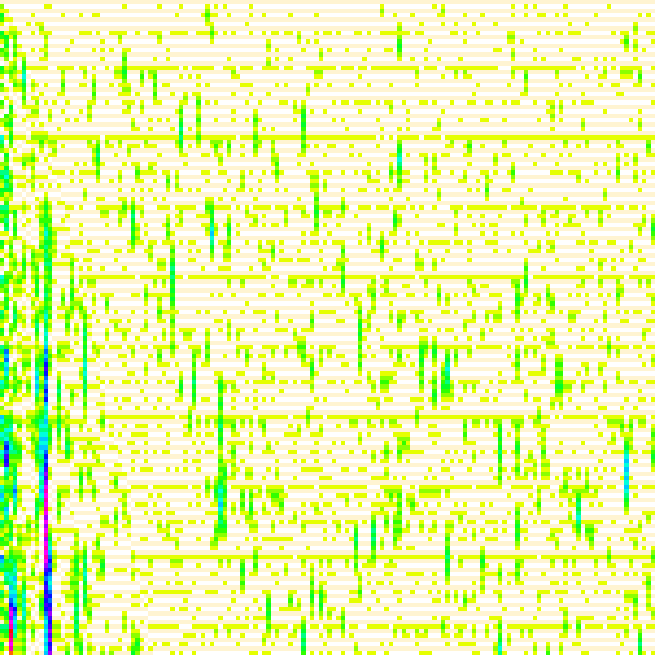
Figure 4.1 expands the above table, plotting piki for 1 ≤ i ≤ 150 and 1 ≤ k ≤ 150 (See Code 4.1 and Code 4.3; Click here for an extended table plotting pi for 1 ≤ i ≤ 150 and 1 ≤ k ≤ 1200):
(Compare to Figure 4.8)
Table 4.1 shows that many primes resonate the multiplicity 2 at kp with k ≡ 0 (mod 16), with lesser resonance for k ≡ 0 (mod 8), and even lesser for k ≡ 0 (mod 4). These show in Figure 4.1 as light green horizontal striations and are likely associated with a standing pattern for p = 2. Following this resonation as k increases, sometimes we see heightened multiplicity descend like “icicles” from the horizontal bands.
We note curious “hotspots”, notably (p, k) = (13, 18), evident in Table 4.1 with its maximum multiplicity 7, and most prominently, (31, 85) maxing out at 11, appearing in a vertical streak of red near the lower left corner, but also the following:
Table 3.6
(p,k) Max
------------
(113,17) 6
(13,18) 7
(487,37) 8
(131,50) 6
(229,54) 8
(7,73) 6
(3,82) 9
(23,88) 8
(31,85) 11
(71,85) 7
(43,90) 6
(2,96) 8
(3,106) 10
(827,109) 8
(31,120) 14
(211,251) 10
(71,284) 14
This is not an exhaustive list; the criteria was a simple visual evaluation of Figure 4.1. The hotspots represent repeated interference of p with other primes, denying the depletion of the register pertaining to p.
The Hotspot Diagonal.
Furthermore, it seems that the prevalence of vertical hotspots somehow respects a diagonal emanating from the origin at (p, k) = (1, 1) that increases in both p and more weakly in k as k increases. (This is evident looking at large at the extended plot of Figure 4.1) Upon closer inspection, this diagonal corresponds to p = k. Fainter “echo” diagonals also appear to the right and perhaps in the denser sector to the left, for the lower values of p. In other words, while k ≤ p, there is greater propensity for multiplicity to trend higher and precipitate a hotspot. Indeed, the occasion where k = p signifies p², which for odd p yields multiplicity 2 in an “unperturbed case”, or one in which the depletion of p puts the oscillation in phase with the unperturbed case. Let's walk through part of the unperturbed state of a register pertaining to odd prime p:
p 1 deposit
2p 0 withdrawal (also from 2)
3p 1 deposit (also to 3)
. .
p^2 2 deposit (only in register p)
p^2+1 1 withdrawal*
p^2+2 0 withdrawal*
p^2+3 1 deposit*
. .
p^3−1 1 deposit*
p^3 4 deposit*
...
(Asterisks indicate alterations to other registers due to prime factors q | k, and we are of course assuming no interference from these other registers).
For odd prime p, for even p ≤ k < p² we have multiplicity 0, and for odd p ≤ k < p² we have multiplicity 1. This implies that when k = p², a necessarily odd number, we deposit 2, which over the ensuing 2 iterations is depleted such that the behavior of the register according to parity of k is reversed. Again, for k = p³, we only have 1 in the register and add 3 to it so that the register stands at 4, which again is drawn down to 0 and reverses the behavior of the register according to parity of k. This leads us to consider what an “unperturbed case” of A008336 might resemble (we shall explore it in the next section). If any entangled prime factor q | k necessitates a deposit and amplifies the register of p, then we have possible grounds for a hotspot. The entangled prime q affects the register of p through the register of q in depletion, triggering the addition of multiplicity in both registers, throwing off the behavior of the register of p according to the parity of k.
We know the axes of Figure 4.1 have (x, y) = (i, k), where k is an integer multiplier that runs through the positives, and i is a prime index. Therefore the axes are not to the same scale, indeed with y affected by the spacing of primes, introducing distortion to the diagonals that might appear. Therefore, we might attempt to rectify Figure 4.1, instead using (x, y) = (pi, k):
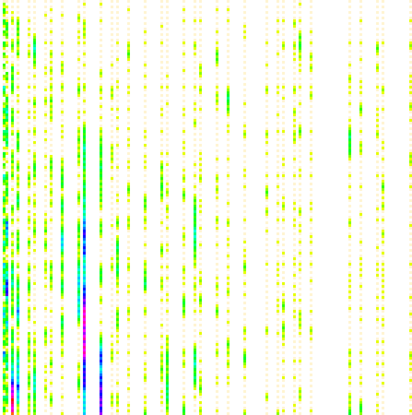
Figure 4.2 applies the same scale to the (x, y) axes, plotting piki for 1 ≤ x ≤ 150 and 1 ≤ k ≤ 150:
(Compare to Figure 4.9)
Figure 4.2 seems to suggest that indeed, along the line k = pi, we see the effect of an amplified register that seems more prone to trigger a hotspot in the wake of that line as k increases. There also seems to be some propensity associated somehow with other bands where k < pi. Zooming out to get more context by an increased range of both k and i, we can generalize
Figure 4.3 extends this plot to (x, y) = (864, 864) and applies red lines at slopes that are positive and negative powers of 2, i.e, the ratio y/x = {16, 8, 4, 2, 1, 1/2, 1/4, 1/8, 1/16} (Click here to see a plot to (x, y) = (1987, 2000)):

We see that these ratios seem to nucleate hotspots; they are not the only cause, but hotspots tend to occur as k increases in the wake of passing these slopes. The phenomenon is perhaps more clearly evident in the extended plot. The association of an amplified occurrence of hotspots with the slopes depicted remains a purely visual observation; investigation is necessary to better define the phenomenon.
The Unperturbed Version of A008336.
Looking at the “unperturbed case” of the registers Ri leads us to try and divine what the corresponding “unperturbed plot” might resemble.
Let us define u(n) as a sequence akin to a(n) in that it alters multiplicity registers Ri pertaining to prime pi according to the condition n | a(n − 1). For a(n), we only debit Ri for pi | n if and only if ALL p | n have sufficient multiplicity stored in their respective registers, otherwise we deposit multiplicity to ALL the respective registers. Of course this is tantamount to the simple definition “if n | a(n − 1), then a(n) = a(n − 1)/n, else a(n) = a(n − 1) × n”, purely based on multiplication or division of a(n − 1) by n. In contrast, for u(n), we debit Ri for all pi | n if sufficient multiplicity is stored in Ri, otherwise we deposit multiplicity in Ri regardless of the state of the registers of other divisors pi | n.
Now let us examine this algebraically, first reviewing the definition of a(n).
Let a(n) be the sequence starting from a(1) = 1 defined as follows:
if n | a(n − 1),
then a(n) = a(n − 1)/n,
else a(n) = a(n − 1) × n.
In contrast, u(n) is a related sequence starting from a(1) = 1 defined as follows:
Let n = p1e1 × p2e2 × … × pkek, and let prime power divisor dk = pkek. Therefore, for all dk | n:
if dk | u(n − 1),
then u(n) = u(n − 1)/dk,
else u(n) = u(n − 1) × dk.
In sum, as regards u(n), we admit the independent modification of a(n − 1) by the prime power divisor dk versus the situation for a(n), where we modify a(n − 1) by n. This allows a more granular modification in the case of u(n), as a partial or split modification of may occur in u(n), while in a(n) the modification must be binary, either n divides or n multiplies a(n − 1). We note that dk < n for n with ω(n) > 1 (i.e., more than a single distinct prime factor). The consequence of this granular versus binary difference is that the moves in a(n) will tend to be greater than those in u(n).
The sequence u(n) begins: (See Code 5.1 and Code 5.2).
{1, 2, 6, 24, 120, 20, 140, 1120, 10080, 1008, 11088, 924, 12012, 858, 1430, 22880, 388960, 1750320, 33256080, 1662804, 3879876, 176358, 4056234, 10816624, 270415600, 10400600, 280816200, ...}
The first discrepancy between the two sequences arises at n = 15 = 3 × 5, with a(15) = 12870 and u(15) = 1430, both arising from a(14) = u(14) = 858. The difference comes about since 3 | 858 but 858 is indivisible by 5. Therefore a(15) = 15 × a(14), but u(15) = 5 u(14) /3. For 15 ≤ n ≤ 20, the register R2 is out of phase between the two sequences; n = 18, depletes R2 in a(n) but credits 2 to R2 in u(n). For n = 21, the depleted R2 in a(n) is recharged to 1, while R2 in u(n) is reduced to 1 from its previous state of 2. Therefore, we have congress between the sequences for 21 ≤ n ≤ 23, ended at n = 24 since 24 does not divide 4056234. Therefore a(24) = 24 × a(23), but u(24) = 8 u(23) /3. For 1 ≤ n ≤ 105, we do not see a(n) = u(n) outside of these 17 terms. Furthermore, the intersection of a(n) and u(n) for is indeed only these 17 terms. It seems plausible, given the prime decomposition of n across the balance of the range, that the intersection of the two sequences is only 17 terms in length.
Table 4.1 compares a(n) and u(n) and their respective multiplicity notations. The zone of intersection between these sequences is hatched:
n a(n) M(a(n)) u(n) M(u(n))
---------------------------------------------------------
1 1 . / / / / / / / / / / 1 .
2 2 1 / / / / / / / / / 2 1
3 6 11 / / / / / / / / / 6 11
4 24 31 / / / / / / / / / 24 31
5 120 311 / / / / / / / / 120 311
6 20 2.1 / / / / / / / / 20 2.1
7 140 2.11 / / / / / / / 140 2.11
8 1120 5.11 / / / / / / / 1120 5.11
9 10080 5211 / / / / / / 10080 5211
10 1008 42.1 / / / / / / / 1008 42.1
11 11088 42.11 / / / / / / 11088 42.11
12 924 21.11 / / / / / 924 21.11
13 12012 21.111 / / / / / 12012 21.111
14 858 11..11 ---------- 858 11..11
15 12870 121.11 1430 1.1.11
16 205920 521.11 22880 5.1.11
17 3500640 521.111 388960 5.1.111
18 194480 4.1.111 1750320 421.111
19 3695120 4.1.1111 33256080 421.1111
20 184756 2...1111 1662804 22..1111
21 3879876 21.11111 ------- 3879876 21.11111
22 176358 11.1.111 / / / / 176358 11.1.111
23 4056234 11.1.1111 ------ 4056234 11.1.1111
24 97349616 42.1.1111 10816624 4..1.1111
25 2433740400 4221.1111 270415600 4.21.1111
26 93605400 3221..111 10400600 3.21..111
27 2527345800 3521..111 280816200 3321..111
28 90262350 152...111 10029150 132...111
29 2617608150 152...1111 290845350 132...1111
30 87253605 .41...1111 9694845 .21...1111
31 2704861755 .41...11111 300540195 .21...11111
32 86555576160 541...11111 9617286240 521...11111
33 2856334013280 551.1.11111 35263382880 511.1.11111
34 84009823920 451.1..1111 1037158320 411.1..1111
35 2940343837200 45211..1111 1452021648 41.11..1111
36 81676217700 23211..1111 3267048708 23.11..1111
...
Additionally, there appear to be only 10 terms where u(n) > a(n), pertaining to n in {18, 19, 20, 50, 51, 52, 53, 54, 55, 56}. We shall see in the ensuing figures, that a(n) grows vastly larger than u(n), the plot of the latter seeming more tempered and true to a logarithmic mean than the former. This seems logical as u(n) depends upon the prime power factors of n, as compared to than n itself.
We can plot u(n) analogous to the plots of a(n).
Figure 4.4 is a log plot of u(n) for 1 ≤ n ≤ 120 akin to Figure 1.1:
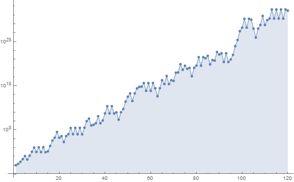
Since we admit divisors d of n with d < n to produce u(n), the sort of order seen in the plot of a(n) in Figure 1.1 is partially missing here.
Figure 4.5 is a log plot that compares a(n) in blue to u(n) in red, for 1 ≤ n ≤ 1000. The effect of the granular moves in u(n) versus the binary moves in a(n) seems to be a more erratic blue line, where a(n) appears to have run away to be very much larger than a(n) as n increases.
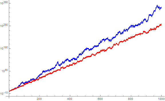
(Compare to Figure 5.2)
Figure 4.6 is a log plot that compares a(n) in blue to u(n) in red, for 1 ≤ n ≤ 10000. Note the smoothness of u(n) compared to a(n).
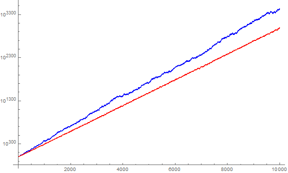
This plot seems to support the fact that the only agreement between the two sequences are those 17 terms, and that aside from these and the 10 terms where u(n) exceeds a(n), a(n) is generally greater than u(n). We surmise (without rigor) this is an effect of the binary moves dependent upon n in a(n), versus the partial and split moves ascribed to prime power divisors of n in u(n), recognizing dk < n for n with more than 1 distinct prime factor.
Figure 4.7 plots 1 ≤ n ≤ 210 on the x axis and the multiplicities in the registers of u(n) on the y axis. The plot is color-coded akin to Figure 3.2. (View a large plot of 1 ≤ n ≤ 214 here.) Compare to Figure 5.3.

Figure 4.8 plots the registers of u(n), piki at (x, y) with x = 1 ≤ i ≤ 150 and y = 1 ≤ k ≤ 150; this is the “unperturbed version” of Figure 4.1:
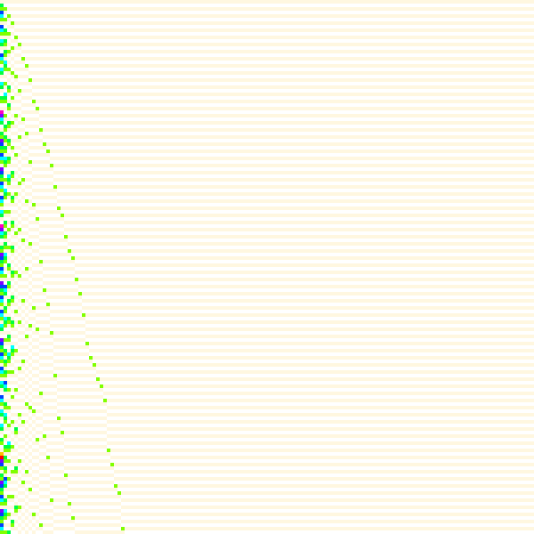
Figure 4.8 seems to clarify that the behavior of the p-registers pertaining to the parity of k, associated with the occasion of perfect powers of p, alternate when the registers are unperturbed by those registers pertaining to other primes. Compare to Figure 5.4.
Figure 4.9: applies the same scale to the (x, y) axes, plotting piki for 1 ≤ x≤ 150 and 1 ≤ k ≤ 150, this is the “unperturbed version” of Figure 4.2:
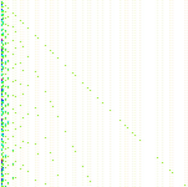
(Compare to Figure 5.5.)
A Related Finer Grain Sequence.
For the sake of thoroughness, we consider a third relative to a(n) and u(n), that of s(n) = A055204(n) of Labos Elemer, the squarefree part of n!. This sequence atomizes the prime decomposition of n into a series of primes with multiplicity p | n.
Let s(n) be the sequence defined as s(1) = 1, and s(n) for n > 1 as follows:
For all prime p | n with multiplicity:
if p | s(n − 1),
then s(n) = s(n − 1)/p,
else s(n) = s(n − 1) × p.
The sequence u(n) for our purposes begins: (See Code 9).
{1, 2, 6, 6, 30, 5, 35, 70, 70, 7, 77, 231, 3003, 858, 1430, 1430, 24310, 12155, 230945, 46189, 969969, 176358, 4056234, 676039, 676039, 104006, 312018, 44574, 1292646, 1077205, 33393355, ...}
We note the intersection of a(n), u(n), and s(n) is {1, 2, 6, 858}, but that there seem to be very many terms common between the latter two sequences, the first of which are {1, 2, 6, 858, 1430, 176358, 4056234, …}. The question of the density of agreement s(n) = u(n) may prove interesting for research. Do these sequences agree more often as n increases or less? The frequency of agreement may become attenuated as n increases, relating to the valuation of n pertaining to large prime divisors as n increases. This subject is beyond the scope of this work.
Table 5.1 compares the three sequences in the fashion of Table 4.1. This table compares a(n), u(n), and s(n) and their respective multiplicity notations. The zones of intersection between a(n) and u(n) and the smallest intersecting terms of u(n) and s(n) are hatched:
n a(n) M(a(n)) u(n) M(u(n)) s(n) M(s(n))
------------------------------------------------------------------------------------
1 1 . / / / / / / / / / / 1 . / / / / / / / / / / 1 .
2 2 1 / / / / / / / / / 2 1 / / / / / / / / / 2 1
3 6 11 / / / / / / / / / 6 11 ----------------- 6 11
4 24 31 / / / / / / / / / 24 31 6 11
5 120 311 / / / / / / / / 120 311 30 111
6 20 2.1 / / / / / / / / 20 2.1 5 ..1
7 140 2.11 / / / / / / / 140 2.11 35 ..11
8 1120 5.11 / / / / / / / 1120 5.11 70 1.11
9 10080 5211 / / / / / / 10080 5211 70 1.11
10 1008 42.1 / / / / / / / 1008 42.1 7 ...1
11 11088 42.11 / / / / / / 11088 42.11 77 ...11
12 924 21.11 / / / / / 924 21.11 231 .1.11
13 12012 21.111 / / / / / 12012 21.111 3003 .1.111
14 858 11..11 ---------- 858 11..11 ---------- 858 11..11
15 12870 121.11 1430 1.1.11 ---------- 1430 1.1.11
16 205920 521.11 22880 5.1.11 1430 1.1.11
17 3500640 521.111 388960 5.1.111 24310 1.1.111
18 194480 4.1.111 1750320 421.111 12155 ..1.111
19 3695120 4.1.1111 33256080 421.1111 230945 ..1.1111
20 184756 2...1111 1662804 22..1111 46189 ....1111
21 3879876 21.11111 ------- 3879876 21.11111 969969 .1.11111
22 176358 11.1.111 / / / / 176358 11.1.111 ------ 176358 11.1.111
23 4056234 11.1.1111 ------ 4056234 11.1.1111 ---- 4056234 11.1.1111
24 97349616 42.1.1111 10816624 4..1.1111 676039 ...1.1111
25 2433740400 4221.1111 270415600 4.21.1111 676039 ...1.1111
26 93605400 3221..111 10400600 3.21..111 104006 1..1..111
27 2527345800 3521..111 280816200 3321..111 312018 11.1..111
28 90262350 152...111 10029150 132...111 44574 11....111
29 2617608150 152...1111 290845350 132...1111 1292646 11....1111
30 87253605 .41...1111 9694845 .21...1111 1077205 ..1...1111
31 2704861755 .41...11111 300540195 .21...11111 33393355 ..1...11111
32 86555576160 541...11111 9617286240 521...11111 66786710 1.1...11111
33 2856334013280 551.1.11111 35263382880 511.1.11111 2203961430 111.1.11111
34 84009823920 451.1..1111 1037158320 411.1..1111 64822395 .11.1..1111
35 2940343837200 45211..1111 1452021648 41.11..1111 90751353 .1.11..1111
36 81676217700 23211..1111 3267048708 23.11..1111 90751353 .1.11..1111
...
Let's look at the behavior of the registers Ri pertaining to prime pi for sequence s(n). These have extremely simple behavior compared to those of a(n) and even u(n), because we may dispense with conditions. Let Ri(n − 1) be any register set to a state, either “on” or “off”, “true” or “false”, etc. but for our purposes 1 or 0, since u(n) is squarefree. Therefore:
For n = p1e1 × p2e2 × … × piei,
Ri(n) = Ri(n − 1) + (ei mod 2) mod 2
Example. Suppose we start with a “light switch” R2 set to off (i.e., 0) for n = 1, and that we only flip the switch if we have a number n that is even, but according to the valuation of the factor 2 in n, that is, for numbers like m = 2, 6, 10, we flip once, since 2 | m, and for 4, 12, 20, since 2² | m, we flip twice, thus resulting in the state the switch was set in the first place, etc.
For n = 2, 2 | 2, thus we flip R2 to “on” (i.e., 1). For n = 3, we do not touch the switch and it remains “on”. For n = 4, since 2² | 4, we flip the switch off-on, and end up with R2 “on”. For n = 5 or any odd, we never touch the switch and its state persists. For n = 6, since 2 | 6, we turn R2 to “off”, where it remains for n = 7. For n = 8, since 2³ | 8, we flip R2 on-off-on, and so it remains “on” for n = 9 only to be switched off at n = 10, etc.
Since the state of nondivisibility does not affect Ri, we only need to regard the parity of the multiplicity of pi | n in order to determine its setting. Thereby, we compute u(n) = p1R1 × p2R2 × … × piRi.
Because s(n) is squarefree, we may interpret its multiplicity notation (reversed as presented in the last column of Table 5.1 above) as a binary number to generate a sequence t(n) that compresses the numbers in s(n) using A067255. Sequence t(n) begins:
0, 1, 3, 3, 7, 4, 12, 13, 13, 8, 24, 26, 58, 51, 53, 53, 117, 116, 244, 240, 250, 235, 491, 488, 488, 457, 459, 451, 963, 964, 1988, 1989, 2007, 1942, 1946, 1946, 3994, 3867, 3897, 3900, 7996, 7991, 16183, 16167, 16163, 15906, 32290, 32288, 32288, 32289, ...
Figure 5.1 is a log plot of s(n) for 1 ≤ n ≤ 120 akin to Figures 1.1 and 4.4:
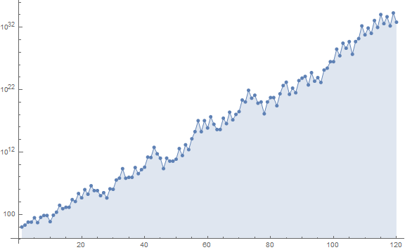
Figure 5.2 is a log plot that compares a(n) in blue, u(n) in red, and s(n) in green, for 1 ≤ n ≤ 1000. We note that s(n) ≤ u(n) as n increases, that s(n) never exceeds u(n) as a consequence of the former sequence dependent upon individual primes p | n (with multiplicity) versus prime power divisors pkek | n, respectively. Therefore s(n) and u(n) are more similar to one another than to a(n).
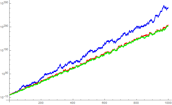
Figure 5.3 plots 1 ≤ n ≤ 210 on the x axis and the multiplicities in the registers of s(n) on the y axis. Since all values are either 0 or 1, we simply represent 1s as black and zeros as white. This is akin to the color plots in Figures 3.2 and 4.7 (View a large plot of 1 ≤ n ≤ 214 here.)

We “unfold” this plot in the next figure, as we have Figure 3.2 into 4.1, and Figure 4.7 into 4.8.
Figure 5.4 plots the registers of s(n), piki at (x, y) with x = 1 ≤ i ≤ 150 and y = 1 ≤ k ≤ 150; analogous to Figures 4.1 and 4.8.
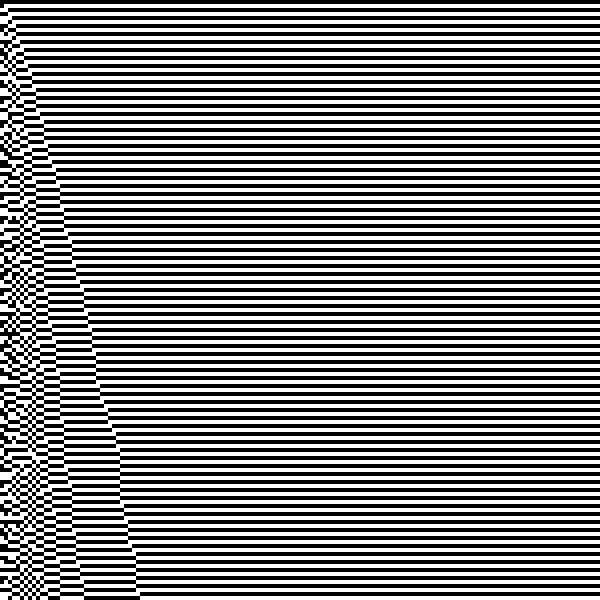
Indeed this is the state of the registers or “light switches” (arranged on the x axis) after the n-th flip, according to valuation as described, that proceed as y increases downward.
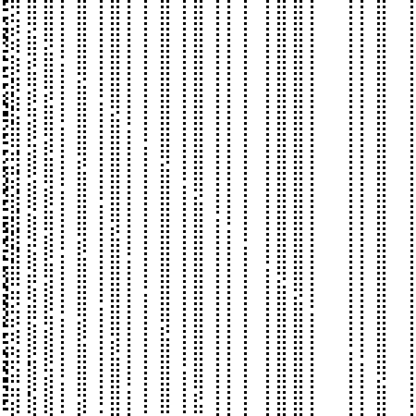
Figure 5.5 applies the same scale to the (x, y) axes, plotting piki for 1 ≤ x ≤ 150 and 1 ≤ k ≤ 150, analogous to Figures 4.2 and 4.9:
Conclusion.
The patterns in Figure 3.4 and its extension, and the connections between a(n), u(n), and s(n) would seem prove to be an interesting subject of a more pointed and rigorous investigation. We have shown that A337486 represents the condition in A008336 relating to divisibility and the necessary downward move of A008336. We have analyzed the behavior of the multiplicities of prime divisors of A008336(n). We have determined that A260850 is an unperturbed version of A008336, where we allow divisors of n to independently modify A260850(n). We have also determined that A055204 is a version of A260850 that allows each prime divisor p | n with multiplicity to modify the previous term rather than prime power factors pk | n for A260850. Thus A055204(n) is never greater than A260850(n), and there are many terms in one that appear in the other at the same index n.
This concludes our examination of OEIS A008336 and the related sequences A055204, A260850, and A337486.
Appendix.
Code 1.1: Generate a(n) = A008336 via Nest:
Nest[Append[#1, If[Mod[#2, #3] == 0, #2/#3, #2 #3]] & @@ {#, #1[[-1]], Length[#]} &, {1, 1}, 10^4]
Code 1.2: Generate A008336 via Do loop:
Block[{nn = 10^4, k = 1}, {1}~Join~Reap[Do[If[Mod[k, i] == 0, k /= i, k *= i]; Sow[k], {i, nn}]][[-1, 1]]]
Code 1.3: Generate b(k) = A337486 via Do loop:
Block[{nn = 10^4, k = 1}, {1}~Join~Reap[Do[If[Mod[k, i] == 0, k /= i, k *= i]; Sow[i], {i, 2, nn}]][[-1, 1]]]
Code 2.1: Examine the multiplicity notation of a(n), where asterisks mark n in b(k), in the fashion of reverse(A054841(a(n)):
Block[{nn = 2^8, p}, Array[Set[p[Prime@ #], 0] &, PrimePi@ nn];
Reap[Do[If[AllTrue[#, p[#1] >= #2 & @@ # &],
Map[p[#1] -= #2 & @@ # &, #];
Sow[{i, "*", StringJoin[Map[ToString[#] /. "0" -> "." &,
Reverse[#][[1 ;; Length[#] - LengthWhile[#, # == 0 &]]] &@
Reverse @ Array[p[Prime@ #] &, PrimePi@nn]]]}],
Map[p[#1] += #2 & @@ # &, #];
Sow[{i, "", StringJoin[Map[ToString[#] /. "0" -> "." &,
Reverse[#][[1 ;; Length[#] - LengthWhile[#, # == 0 &]]] &@
Reverse@ Array[p[Prime@ #] &, PrimePi@ nn]]]}]
] &@ FactorInteger[i], {i, 2, nn}]][[-1, 1]]] // TableForm]
Code 3.1: Plot the multiplicity notation of a(n), marking n in b(k) with a black tick mark at bottom. Note that the concatenated form of multiplicity notation is subject to possible ambiguosity in the case of a multiplicity exceeding 9. Per Table 3.4, this code avoids such for nn < 308:
Block[{nn = 300, p, k = 6, o = 2.5, v, m},
m = If[nn > 4040, 28,
SelectFirst[{{1, 1}, {3, 3}, {7, 5}, {63, 7}, {191, 8}, {242, 9}, {308, 10}, {314, 11}, {503, 12},
{704, 13}, {719, 14}, {724, 16}, {749, 17}, {754, 18}, {799, 19}, {2753, 23}, {2756, 24},
{2816, 25}, {4031, 26}, {4034, 27}, {4040, 28}},
First@ # > nn &][[-1]] ];
Array[Set[p[Prime@# ], 0] &, PrimePi@ nn];
v = Reap[Do[If[AllTrue[#, p[#1] >= #2 & @@ # &],
Map[p[#1] -= #2 & @@ # &, #];
Sow[Join @@ {ConstantArray[Black, k], ConstantArray[White, k],
Array[If[# == 0, White, Hue[(# + o)/m,
If[# > 1, 1, (# + o)/m]]] &@ p[Prime@ #] &, PrimePi@ nn]}],
Map[p[#1] += #2 & @@ # &, #];
Sow[Join @@ {ConstantArray[White, 2 k],
Array[If[# == 0, White, Hue[(# + o)/m, If[# > 1, 1, (# + o)/m]]] &@ p[Prime@ #] &, PrimePi@ nn]}]
] &@FactorInteger[i], {i, 2, nn}]][[-1, 1]];
Image[Transpose@ Map[Reverse, v], ColorSpace -> "HSB"]]
Code 4.1: Generate a prime-modular-adjusted tabular dataset* to support tables and plots like Table 3.4 and Figure 4.1:
* Note: the settings as written require about five minutes to generate a dataset. To select a smaller rectangle, first divide nn/prime( j) to give the maximum number of rows, k, that can be accommodated.
Block[{nn = 2^20, j = 150, k = 1200, p, s},
Array[Set[p[Prime@ #], 0] &, PrimePi@ nn];
s = Reap[Do[
If[AllTrue[#, p[#1] >= #2 & @@ # &],
Map[p[#1] -= #2 & @@ # &, #]; Sow@ Array[p[Prime@ #] &, j],
Map[p[#1] += #2 & @@ # &, #]; Sow@ Array[p[Prime@ #] &, j]
] &@ FactorInteger[i], {i, 2, nn}]][[-1, 1]];
Transpose@
MapIndexed[Function[{a, p},
Map[a[[#]] &, Range[p - 1, nn - 1, p] ][[1 ;; k]] ] @@
{#1, Prime@ First[#2]} &, Transpose[s][[1 ;; j]]]]
Code 4.2: Generate a table akin to Table 4.1 (set Code 4.1, nn = 2^13, j = k = 36, run Code 4.2 after Code 4.1):
Prepend[MapIndexed[Prepend[#1, First[#2]] &, #],
Prepend[Prime@ Range[Length@ #[[1]] ], {}]] &@ % // TableForm
Code 4.3: Generate a plot akin to Figure 4.1 (run Code 4.1 as written first):
With[{o = 2.5, m = Max@ #},
Magnify[#, 4] &@
Image@ Map[If[# == 0, White, Hue[(# + o)/m, If[# > 1, 1, (# + o)/(m - 5)]]] & /@ # &, #]] &@ %
Code 5.1: Generate A260850 using registers, via Do loop::
Block[{nn = 33, p, lim}, lim = PrimePi@ nn;
Array[Set[p[Prime@ #], 0] &, PrimePi@ nn];
Reap[Do[(Map[If[p[#1] >= #2, p[#1] -= #2, p[#1] += #2] & @@ # &, #];
Sow[Times @@ Array[#^p[#] &@ Prime@ # &, lim]]) &@
FactorInteger[i], {i, nn}]][[-1, 1]]]
Code 5.2: Generate A260850 using arithmetic, via Do loop::
Block[{nn = 40, k = 1},
Reap[Do[Map[If[Mod[k, #] == 0, k /= #, k *= #] &,
Flatten[ConstantArray[#1, #2] & @@@ FactorInteger@ i]];
Sow[k], {i, nn}]][[-1, 1]]]
Code 5.3: Generate A055204 using registers, via Do loop::
Block[{nn = 40, k, p}, k = PrimePi@ nn;
Array[Set[p[Prime@ #], 0] &, k];
{1}~Join~Reap[Do[Map[Set[p[#1], Mod[p[#1] + Mod[#2, 2], 2]] & @@ # &, FactorInteger@ i];
Sow[Times @@ Array[#^p[#] &[Prime[k - # + 1]] &, k], 2], {i, 2, nn}]][[-1, 1]]]
Code 5.4: Generate A055204 using arithmetic, via Do loop::
Block[{nn = 40, k = 1},
Reap[Do[Map[If[Mod[k, #] == 0, k /= #, k *= #] &,
Flatten[ConstantArray[#1, #2] & @@@ FactorInteger@ i]];
Sow[k], {i, nn}]][[-1, 1]]]
Extended Tables.
Record transform of a(n) = A008336. The records are in r(k) and indices in s(k), reckoned per this paper. To obtain the OEIS indexing, add 1 to s(k). M(r(k)) is the multiplicity notation of r(k), here used to analyze the prime decomposition of r(k) in a succinct way. This link extends the table below to k = 120. (See Code 4.)
k s(k) r(k) M(r(k))
----------------------------------------
1 1 1 .
2 2 2 1
3 3 6 11
4 4 24 31
5 5 120 311
6 7 140 2.11
7 8 1120 5.11
8 9 10080 5211
9 11 11088 42.11
10 13 12012 21.111
11 15 12870 121.11
12 16 205920 521.11
13 17 3500640 521.111
14 19 3695120 4.1.1111
15 21 3879876 21.11111
16 23 4056234 11.1.1111
17 24 97349616 42.1.1111
18 25 2433740400 4221.1111
19 27 2527345800 3521..111
20 29 2617608150 152...1111
21 31 2704861755 .41...11111
22 32 86555576160 541...11111
23 33 2856334013280 551.1.11111
24 35 2940343837200 45211..1111
25 37 3022020054900 23211..11111
26 39 3101546898450 142111..1111
27 40 124061875938000 443111..1111
28 41 5086536913458000 443111..11111
29 43 5207644935207000 333.11..111111
30 49 6320530321887600 4222.1...111111
31 51 6446940928325352 33.2.11..111111
32 53 6570920561562378 13.2..1..1111111
33 55 6692604275665385 ..121.1..1111111
34 56 374785839437261560 3.131.1..1111111
35 57 21362792847923908920 31131.11.1111111
36 59 21731116862543286660 21131.11..1111111
...
Concerns sequences:
A002110: Primorials; products of the smallest n primes.
A008336: a(n).
A054841: Multiplicity notation: Write n = p1k1 × p2k2 × … × pmkm as concatenation of {km, …, k2, k1}.
A055204: s(n) = squarefree part of n!.
A067255: Multiplicity notation: Write n = p1k1 × p2k2 × … × pmkm as {k1, k2, …, km}.
A260850: u(k).
A336510: t(n) = Sum_{p | A055204(n)} 2^(π(p) − 1).
A337486: b(k).
This work is dedicated to my mother Mauricia, native of Guiuan, Eastern Samar, Philippines, on the near occasion of her 78th birthday.
Document Revision Record.
2020 0912 2245 Created.
2020 0914 2200 Added tables and figures.
2020 0916 1730 Connection to A260850.
2020 0916 2145 Code 9 added.
2020 0917 1230 Connection to A055204.
2020 0918 1545 Abstract, posed A336510(n) = t(n).