Icarus Revisited.
A sequence of David Sycamore.
Written by Michael Thomas De Vlieger, St. Louis, Missouri, 2021 0408.
Abstract.
We examined a nested doubly conditional self-referential sequence with contramanding counting functions that produces two major canonical nontrivial trajectories, based on primality (see s20210303). This sequence produced finite trajectories. In this paper we explore such a sequence based on squares to attempt to prolong the trajectories.
Introduction.
This paper describes a doubly conditional self-referential recursive mapping h(x), where x ≥ 0 is an integer used as a seed. The recursive mapping of h(x) produces an infinite sequence, however, there is a mechanism that eventually arises given any x that results in a fixed point of 0.
The map h(x) produces a sequence beginning with sx(0) = x, incrementing thereafter n times. We subject the term x to Condition A, a novelty test, and in both outcomes, to Condition B that determins if x is a perfect square, yielding output based on the four possible overlaid conditions. The output serves as input for another mapping until we encounter two adjacent zeros (a fixed point of 0). We say a number m is novel if it does not already appear in s, and extant if it already appears at least once at s(k) for k < n. We will use the term “square” to mean n such that √n is an integer, and “nonsquare” otherwise.
Therefore, we define a sequence sx starting with sx(0) = x.
For novel square s(n), we report the number c of squares m in s at s(n+1).
For novel nonsquare s(n), we report the number (n − c) of nonsquares m in s at s(n+1).
For extant square s(n) whose penultimate index is k, we write at s(n+1) the number of nonsquares in s(j), k < j < n.
For extant nonsquare s(n) whose penultimate index is k, we write at s(n+1) the number of squares in s(j), k < j < n.
Conditional structure of s.
There are 4 practical conditions, to which we assign labels.
- Condition 0 pertains to novel nonsquare m wherein we do not increment c, and enter s(n+1) = (n − c).
- Condition 1 pertains to novel square m wherein we increment c and enter s(n+1) = c.
- Condition 2 pertains to extant nonsquare m seen at s(k), k < j < n, wherein we do not increment c but report the number of square s(j).
- Condition 3 pertains to extant square m seen at s(k), k < j < n, wherein we increment c and report the number of nonsquare s(j).
We use these conditions to produce an auxiliary sequence r that tracks the condition enacted during each iteration.
The general effect of Conditions 0 and 1 (the novel conditions) is to introduce the status of c or (n − c) at s(n+1) if and only if m is novel. Since there are more nonsquares than squares in the intervals dealt with during generation, the trajectory of (n − c) proves higher and more continuous than that of c in the scatterplot of s. Each time Condition 0 or 1 occurs, the respective counting function has strictly increased. Therefore, generally, the emergence of these conditions has a sustaining effect upon the duration of a nontrivial run of s. Using the analogy of Icarus, these two conditions perhaps represent his flight, maybe a bit too close to the sun.
The general effect of Conditions 2 and 3 (the extant conditions) is to report the number of integers in the interval between the latest 2 instances of m with opposite “squareness” at s(n+1). Hence, Condition 3 (pertaining to extant squares) tends to report larger numbers of nonsquares more infrequently than Condition 2 reports smaller numbers of squares. Condition 2 tends to be the reason that forces s into a fixed point through instigating 2 adjacent zeros. Again, the analogy of Icarus has us consider these conditions as Icarus’ fateful accumulation of sea-spray until he crashes into the Aegean.
In comparison to a similar function that depends on primality rather than “squareness”, The difference between the square counting function and the nonsquare counting function is more pronounced.
Generation of sequence s.
We now examine three examples of the recursive mappings of h(x) given seeds 2 and 9. In all cases, we set s(0) = seed.
s2 begins:
2, 1, 1, 0, 3, 2, 3, 0, 3, 1, 4, 6, 6, 0, 3, 3, 0, 2, 5, 11, 12, 13, 14, 15, 16, 9, 10, 17, 18, 19, 20, 21, 22, 23, 24, 25, 11, 3, 4, 22, 2, 4, 2, 1, 25, 5, 7, 32, 33, 34, 35, 36, 16, 20, 7, 2, 4, 10, 8, 41, 42, 43, 44, 45, 46, 47, 48, 49, 19, 9, 34, 5, 5, 0, 44, 3, 10, 3, 0, 4, 18, 13, 15, 15, 0, 4, 4, 0, 0, ...
s2(1) = 1 since s2(0) is new to s and not a perfect square, and there is 1 nonsquare in the sequence.
s2(2) = 1 since s2(1) is new to s and is a perfect square; there is 1 square in the sequence.
s2(3) = 0 since s2(2) is a square that appeared at s1(1); between s1(1) and s1(2) there no nonsquares.
s2(4) = 3 since s2(3) is a novel square, and there 3 squares in the sequence.
s2(5) = 2 since s2(4) is a novel nonsquare, and there are 2 nonsquares in the sequence.
s2(6) = 3 since s2(5) is a nonsquare that appeared at s1(0); between s1(0) and s1(5) there are 3 squares.
...
For n > 88, we will always have 0 since there are no nonsquares between adjacent zeros, and the sequence is hereinafter trivial. Hence, we may speak of a nontrivial run length ℓ, the number of iterations necessary to produce 2 adjacent zeros. Therefore, ℓ2 = 88. This pattern pertains to an infinite number of nonsquares and has 31 defects.
s9 begins:
9, 1, 2, 1, 1, 0, 5, 2, 3, 4, 6, 5, 1, 5, 1, 1, 0, 6, 4, 4, 0, 1, 1, 0, 0, ...
Run length ℓ9 = 24. This pattern pertains to an infinite number of squares and has 3 defects.
We see that there are 2 principal conditions of such sequences s, based upon the nature of the seed, seeing s(1) = 1 for any input. Given a square seed x = S, we have {S, 1, 2, …}, and a nonsquare seed x = N, we have {N, 1, 0, …}. The exception to the square seed pattern is x = 1, resulting in {S, 1, 0, …}.
Defects arise in the S and N trajectories when x conflicts with the same x that arises later in the trajectory. The conflict involves converting a novel to an extant progenitor s(n), normally resulting in a vastly different report at s(n+1). A key consideration is that the novelty test when positive requires reporting the number c or (n − c), with c incrementing upon the occasion of both novel and extant squares, granting opportunities for gaps in the reporting of the counting functions c or (n − c) through which certain seeds x pass, so as not to disturb the canonical sequence.
Canonical Trajectories.
There are 2 “canonical trajectories” that derive from the 4 possible conditional states that govern the sequence s. These include the novel nonsquare (NN) and the novel square (NS) canonical trajectories pertaining to conditions 0 and 1, respectively. There can be no “extant” trajectory (X) since any seed is unprecedented in s.
For all x, we have s(1) = 1, since s(0) = x is novel. Regardless of whether or not x is square, for n = 1, there is 1 instance of the appropriate species (nonsquare or square) in s. If x is square, then s(2) = 2 else s(2) = 0.
The Canonical Square Trajectory.
Let us consider a square seed x, supposing it is a square S that does not interfere with any element in the trajectory. We produce a pattern sS as follows:
Figure 1: The color function shows sS(n) with novel square progenitors in red, novel nonsquare progenitors in yellow, extant square progenitors in blue, and extant nonsquare progenitors in green. The ringed figures highlight the point of departure for the seed x written below. The nonsquare pattern departs at the term under which a black dot appears.

Figure 2 is an annotated scatterplot of sS = s9:
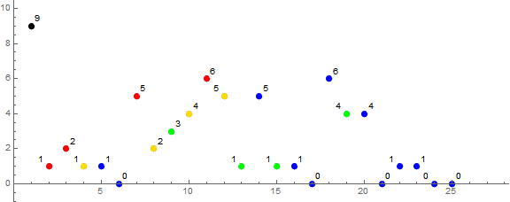
The plot shows the first 2 trivial zeros.
The death knell appears to be the instance of two adjacent extant numbers that are both nonsquare, followed by two zeros.
The Canonical Nonsquare Trajectory.
Let us consider a nonsquare seed x, supposing it is a number N that is not a perfect square and does not interfere with any element in the trajectory. We produce a pattern sN as follows:
Figure S2: The color function shows sN(n) with novel square progenitors in red, novel nonsquare progenitors in yellow, extant square progenitors in blue, and extant nonsquare progenitors in green. The ringed figures highlight the point of departure for the seed x written below. The square pattern departs at the term under which a red dot appears. The seed x = 2 is circled, however, 2 does not spur a trajectory that differs from sN since the result of the novel and extant conditions is the same at n = 2.
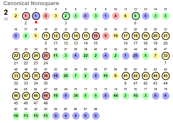
This trajectory has length ℓN = 88 and first arises for N = 2. We find that if ever N does appear in sN , it induces a departure from this canonical nonsquare trajectory. This is because, for x = N, N already appeared at k = 0, therefore its appearance at n is its second appearance, meaning it is now an extant nonsquare, triggering Condition 2 instead of Condition 0. It could be possible to end up with the canonical sequence anyway. For that to happen, Condition 2 would yield the same s(n) as Condition 0. There are only 31 conflicting nonsquare seeds and all have been observed to deviate from the canonical nonsquare trajectory.
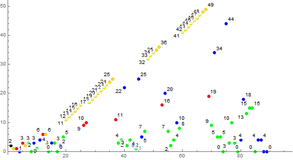
The seed x = 2 does interact with s(5) = 2, however, Condition 0 and 2 have the same effect: (n − c) = number of s(j) for 0 < j < 5 = 3, therefore there is no difference between the trajectory of s2 and the canonical nonsquare trajectory (hence the reason for s2 being the first instance of the canonical trajectory).
Figure 4 is a scatterplot of s2:
Transmissivity of the Canonical Trajectories.
Let us examine the canonical trajectories to determine the gaps in coverage that serve as “holes” in the multiset through which seeds x may pass without disturbing any element in the trajectory.
For the canonical square trajectory s9, we have ℓ9 = 24 with the maximum (excepting seed) s9(10) = s9(17) = 6. The numbers 0 through 6 inclusive appear in s9, which means that the square seeds {0, 1, 4} interact with a term in the canonical trajectory.
For seed x = 0, we have a collision with s(5) = 0, with resulting ℓ = 8.
For seed x = 1, we have a collision with s(1) = 1, with resulting ℓ = 9.
For seed x = 4, we have a collision with s(9) = 4, with a lengthened ℓ = 548.
All other square seeds have the canonical pattern with ℓ = 24, since all squares S > 6 exceed any term in the canonical pattern and do not interact with the trajectory.
For the canonical nonsquare trajectory s2, we have ℓ2 = 88 with the maximum s2(68) = 49. The follwing numbers less than 49 do not appear in the canonical trajectory:
26, 27, 28, 29, 30, 31, 37, 38, 39, 40
Therefore, these and any nonsquare seeds x > 49 follow the canonical nonsquare trajectory, as they do not interact with any term in the canonical trajectory. The seed x = 2 does interact with s(5) = 2, as shown in the previous section. Thus we have the following nonsquare seeds x that depart from the canonical trajectory:
3, 5, 6, 7, 8, 10, 11, 12, 13, 14, 15, 17, 18, 19, 20, 21, 22, 23, 24, 32, 33, 34, 35, 41, 42, 43, 44, 45, 46, 47, 48
We observe that there are fewer departures from canon in this variant of s, compared to the primality variant.
The Effect of Defection from Canon.
The canonical trajectories are those that allow the sequence sS or sN to progress unimpeded by collision with a square seed x = S or a nonsquare seed x = N. The collisions affect the first appearance of x in the canonical trajectory s, transmuting its conditional mode from a novel to an extant square or nonsquare.
The transmutation of a novel nonsquare to an extant nonsquare necessitates the application of Condition 2 (green) in place of Condition 0 (yellow). Therefore, instead of reporting the number (n − c) of nonsquares in s, we report the number qS of squares between s(k) and s(n). The number (n − c) increases quite rapidly and more often, whereas qS tends to be a “random” yet relatively small number. The later the interaction of seed x with its appearance in the canonical nonsquare trajectory, the greater the tendency to “kill” the flight of Icarus.
The transmutation of a novel square to an extant square necessitates the application of Condition 3 (blue) in place of Condition 1 (red). Therefore, instead of reporting the number c of squares in s, we report the number qN of nonsquares between s(k) and s(n). The number c increases mildly, whereas qN tends to be a “random” and widely scattered number.
As regards the 3 square collisions {0, 1, 4}, two seeds {0, 1} result in a shortened run length (8 and 9 iterations vs. canonical 24) and x = 4 prolonged flight to ℓ2 = 544 iterations.
Regarding the 32 nonsquare collisions, x = 2 and x = 6 enjoy collisions without effect and presents the canonical nonsquare trajectory of ℓN = 88 iterations. Three seeds {7, 32, 42} result in shortened run lengths, 60, 40, and 81 respectively. Ten seeds have run lengths in the hundreds and 10 seeds have run lengths in the thousands. Seven seeds have run lengths in the ten-thousands, in order least to greatest run length: {47, 5, 20, 18, 15, 3, 10}, the longest of which is ℓ10 = 75392 iterations.
Hence we may write a sequence L with offset 0 containing the run lengths of seeds n:
8, 9, 88, 73646, 548, 11180, 88, 60, 104, 24, 75392, 3483, 6927, 2740, 6291, 21085, 24, 136, 13116, 200, 12876, 437, 864, 40, 113, 24, 88, 88, 88, 88, 88, 88, 4599, 4349, 103, 293, 24, 88, 88, 88, 88, 3756, 81, 117, 6156, 143, 2939, 10634, 2254, 24, 88, 88, 88, 88, 88, 88, 88, 88, 88, 88, ...
Thereafter, we write 88 for nonsquare n and 24 for square n.
There doesn’t appear to be a pattern among the defective seeds that would either predictably prolong or reduce the flight of Icarus.
We remark that the run lengths of certain nonsquare seeds greatly exceeds those of the primality variant of s. Also compared to the primality variant, the dominant mode of instigation in prolonged seed trajectories is Condition 0. That condition is even more dominant in this variant than in the primality variant.
The Tree of Icarus’ Trajectories.
We can plot a tree of all the possible trajectories s by bringing together the sequence condition diagrams for all 34 distinct seeds x, rendered in a linear fashion. This was conducted for the primality variant, where the run lengths were much shorter. It is possible to do the same for this sequence, however the graph would require over 75,000 pixels and thus we have not conducted the same study here.
Daedalus gamed out all of King Minos' schemes to bring his boy down, out of the sky and into the Aegean. Hence he found a way to force more assymmetry into h(x) by selecting a function that rarified instances of a positive register. He substituted the status of perfect squareness rather than primality. When he tested that new function, Icarus was able to fly for longer strides of Condition 0. As a matter of fact, indeed, Icarus' flight was much longer under the new function. Alas, it was not sufficient to have the boy fly forever. We continue to fight the propensity of the extant conditions to pull Icarus down from the novel flight path and into the sea.
Appendix:
Table A: Aggregate data for each trajectory.
Column “x” pertains to seed x; “State” to whether x is square: s denotes square, n nonsquare.
Column “ℓ” is the nontrivial run length of sx, while D is the index of x in the canonical trajectory.
The
“Modes” section counts the conditions that appear in sx. c0 pertains to novel nonsquares, c1 to novel squares, c2 to extant nonsquares, and c3 to extant squares.
The
“Maximum” section pertains to the largest term in sx, listing the maxima and their indices.
The
“Last” section regards the last nontrivial term in sx, listing the term and the instigating condition.
| Modes | Maximum | Last
| NN NS XN XS | |
x States ℓ D c0 c1 c2 c3 max position last c
-------------------------------------------------------------------------------
(2) n 88 5 32 8 29 20 49 68 4 4
3 n 73646 4 70986 270 1947 444 72900 73600 4 4
5 n 11180 18 9741 104 1057 279 10609 10933 0 4
(6) n 88 11 32 8 29 20 49 68 4 4
7 n 60 46 19 6 19 17 25 {36,45,51} 4 4
8 n 104 58 24 7 45 29 36 52 4 4
10 n 75392 26 72113 273 2445 562 74529 75352 4 4
11 n 3483 19 2418 56 776 234 3136 3406 4 4
12 n 6927 20 5221 78 1260 369 6241 6615 4 4
13 n 2740 21 2082 50 456 153 2500 2689 4 4
14 n 6291 22 4952 74 990 276 5929 6271 4 4
15 n 21085 23 18625 143 1836 482 20449 21066 4 4
17 n 136 27 58 9 43 27 81 105 4 4
18 n 13116 28 10157 109 2276 575 12321 12967 9 4
19 n 200 29 104 13 50 34 144 179 4 4
20 n 12876 30 10580 107 1754 436 12100 12577 4 4
21 n 437 31 182 18 171 67 289 348 0 4
22 n 864 32 596 27 178 64 676 730 9 9
23 n 99 33 35 6 35 24 47 74 0 1
24 n 113 34 32 8 48 26 64 {85,108,110} 0 1
32 n 4599 47 4002 67 417 114 4356 4513 4 4
33 n 4349 48 3864 64 313 109 4096 4239 0 9
34 n 103 49 45 8 29 22 64 83 9 9
35 n 293 50 158 15 81 40 225 272 4 4
41 n 3756 59 3145 59 416 137 3364 3489 4 4
42 n 81 60 30 8 24 20 49 71 9 9
43 n 117 61 30 8 52 28 49 69 4 4
44 n 6156 62 4338 72 1348 399 5476 5884 4 4
45 n 143 63 48 10 52 34 100 136 16 64
46 n 2939 64 1724 47 907 262 2601 2893 9 1
47 n 10634 65 9322 100 965 248 10201 10525 4 4
48 n 2254 66 1423 43 596 193 1849 2023 0 4
-------------------------------------------------------------------------------
0 s 8 5 1 2 0 6 2 3 0 1
1 s 9 1 1 2 0 7 3 4 0 1
4 s 548 9 187 17 239 106 324 402 1 1
Figure A4: Scatterplot of s4, a distinct trajectory that defects from the canonical square trajectory s2 at n = 10, by influence of 4 being present in the trajectory s9. The initial instance of x = 4 transmutes s(9) to an extant square rather than novel. This alteration increases the longevity of a square-seeded trajectory to run lenght ℓ4 = 548 vs ℓ2 = 24. The color function addresses the condition instigating the term. Gold indicates a preceding novel nonsquare, red a preceding novel square. Green indicates a preceding extant nonsquare, and blue indicates a preceding extant square.
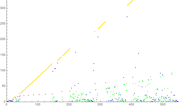
Figure A12: Scatterplot of s12, a distinct trajectory that defects from the canonical nonsquare trajectory s2 at n = 21, by influence of 12 being present in the trajectory s2. The initial instance of x = 12 transmutes s(20) to an extant nonsquare rather than novel. This alteration imparts maximum longevity to : ℓ12 = 6927 vs ℓ2 = 88. The color function is explained in Figure A4.
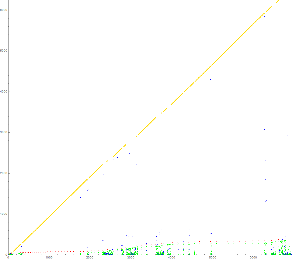
Figure A3: Scatterplot of s3, a distinct trajectory that defects from the canonical nonsquare trajectory s2 at n = 5, by influence of 4 being present in the trajectory s2. The initial instance of x = 3 transmutes s(4) to an extant nonsquare rather than novel. This alteration imparts maximum longevity to : ℓ3 = 73646 vs ℓ2 = 88. The color function is explained in Figure A4.
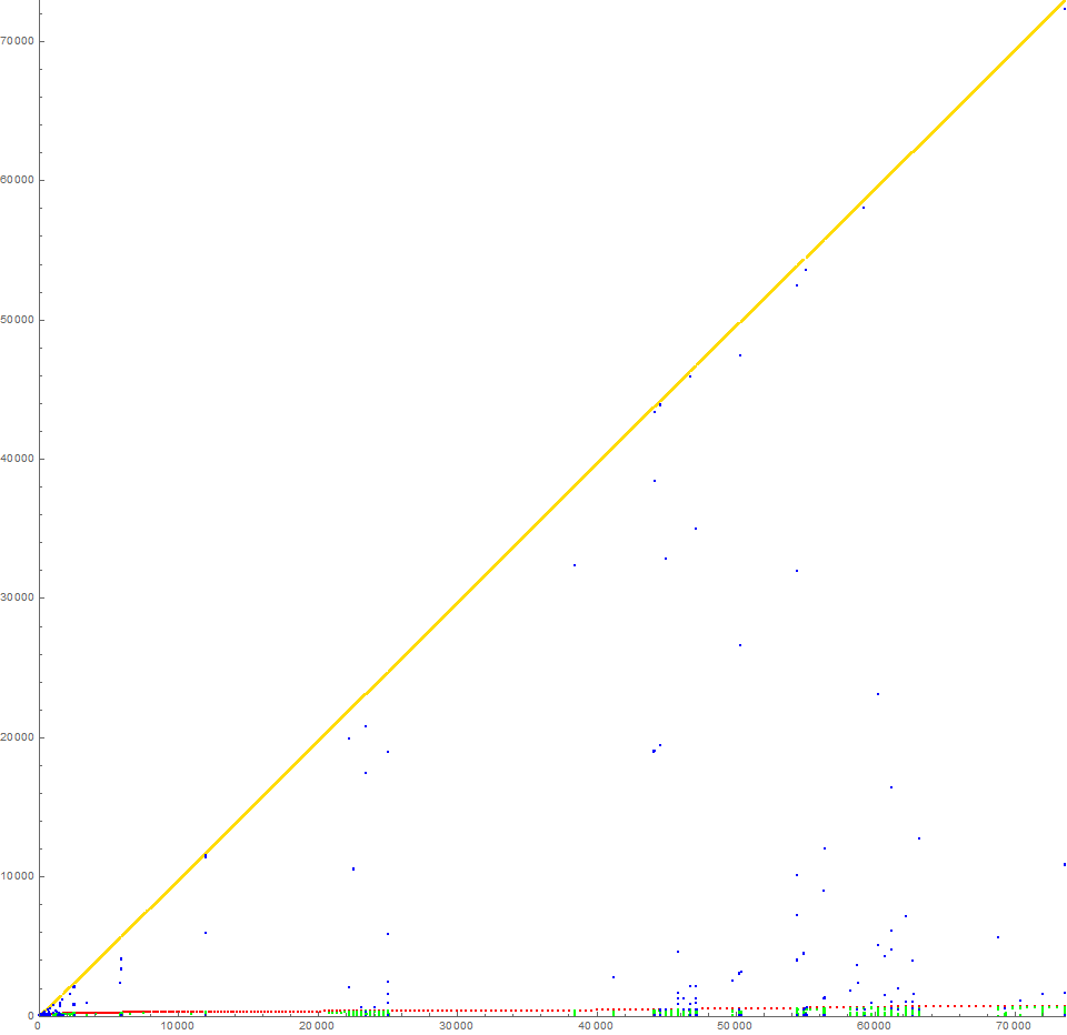
Figure A10: Scatterplot of s10, a distinct trajectory that defects from the canonical nonsquare trajectory s2 at n = 27, by influence of 10 being present in the trajectory s2. The initial instance of x = 10 transmutes s(26) to an extant nonsquare rather than novel. This alteration imparts maximum longevity to : ℓ10 = 75392 vs ℓ2 = 88. The color function is explained in Figure A4. Click here for an enlarged scatterplot.

Block[{a = {2}, c = 0},
Monitor[Do[If[And[i > 2, a[[-2 ;; -1]] == {0, 0}], Break[],
If[FreeQ[Most@ a, #],
If[IntegerQ@ Sqrt[#],
c++; AppendTo[a, c],
AppendTo[a, i - c]],
If[IntegerQ@ Sqrt[#],
c++; AppendTo[a,
Count[a[[-FirstPosition[Reverse@ Most@ a, #][[1]] ;; -2]],
_?(! IntegerQ@ Sqrt[#] &)] ],
AppendTo[a,
Count[a[[-FirstPosition[Reverse@ Most@ a, #][[1]] ;; -2]],
_?(IntegerQ@ Sqrt[#] &)] ]]
] &@ a[[-1]] ], {i, Infinity}], i]; a]
Document Revision Record.
2021 0410 0930 Publication.
2021 0410 1515 Aggregate data, large scatterplots.